EOL: Accordion Agent Q1 - User Manual

Introduction

AGENT™ is a versatile test- and automation platform for a wide range of applications, including test interface, automated machine control systems and data logger.

The base unit provides I2C, JTAG, SPI and UART communication as well as 32 channel Fixture control I/Os and fan control.

Modules can be added to expand capacity up to 192 measurement channels through the on-board IDC connectors. Additional expansion slots are also available.

Real linux-based computer system offers modern connectivity and a wide range of possible on-board functionality.

Accordion AGENT™

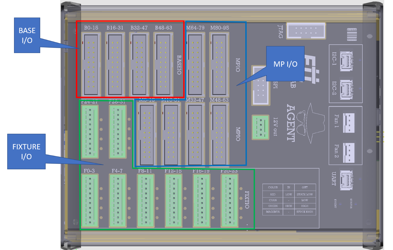
AGENT™ I/O

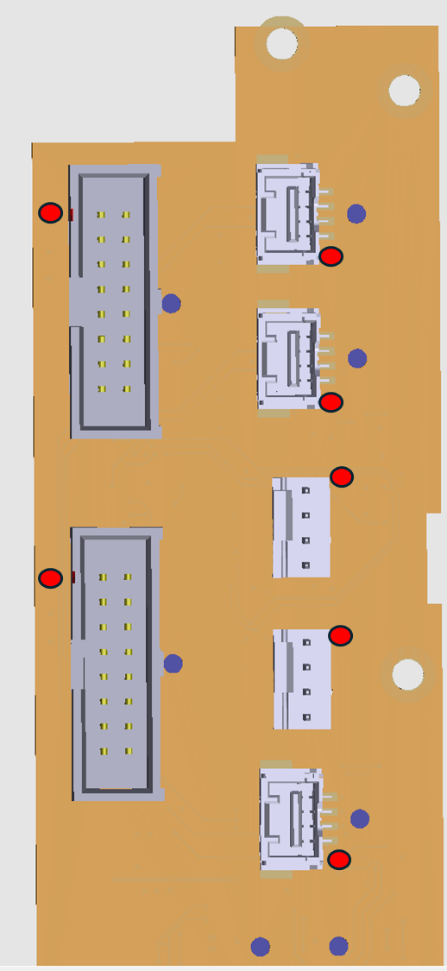
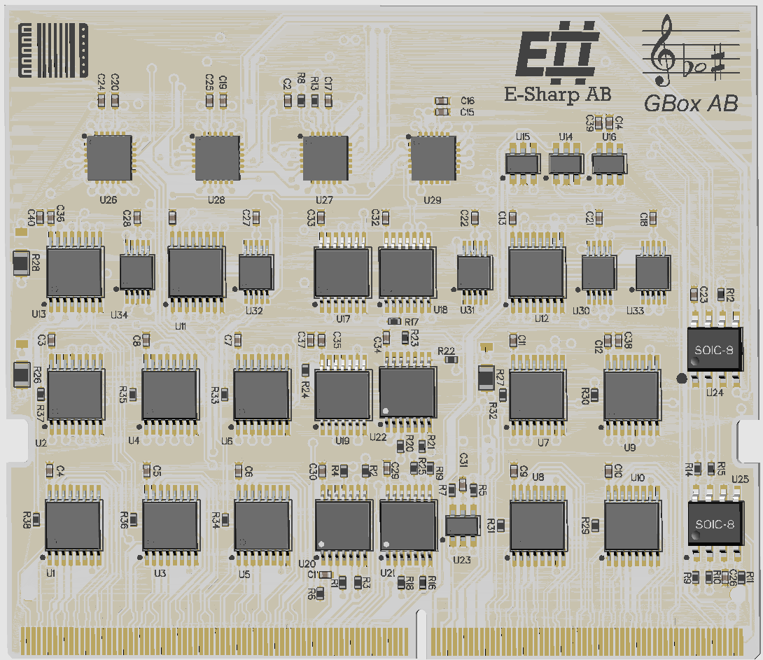
AGENT™ is built with 18 input/output connectors. Pin numbers and specifications of each contact are described below.

Pin numbers

Pin number 1 is marked with a black dot.

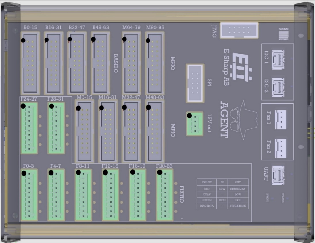
Figure 1 AGENT pin numbers

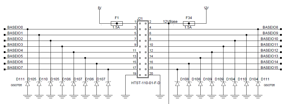
Base I/O

From the expansion slot placed on the base board (slot A4, the name of the channels will start with 0.4.[…]), 64 signals are routed to the connectors called “BASE I/O”.

There are a total of 4 connectors on the AGENT. Each base I/O contact consists of a total of 20 pins. Pin 1 is connected to 5V and pin 2 is connected to 12V. Pins from 3 to 18 are the 16 input/output pins. Pin 19 and 20 are connected to ground.

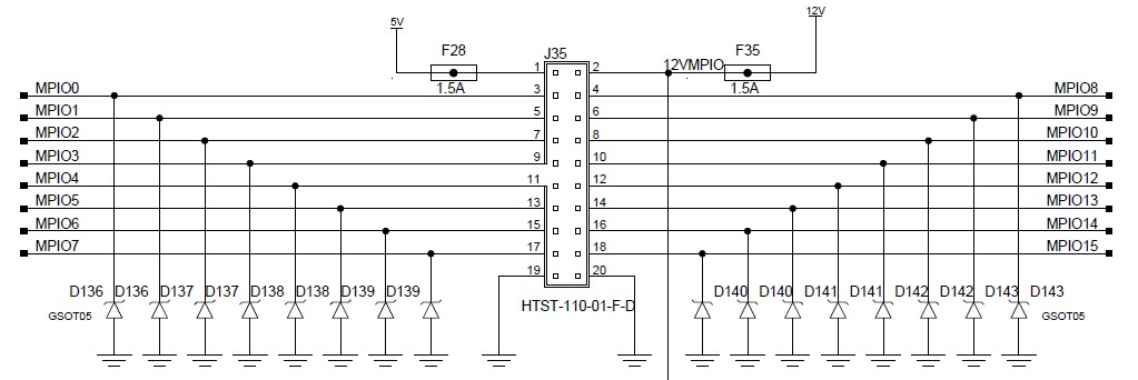
MultiPurpose I/O

From the expansion slot placed on the top board, 96 signals are routed to the connectors called “MPIO”. The name of the channels will start with 0.8.[…]

There are a total of 6 contacts on the AGENT. Each MPIO contact consists of a total of 20 pins. Pin 1 is connected to 5V and pin 2 is connected to 12V. Pins from 3 to 18 are the 16 input/output pins. Pin 19 and 20 are connected to ground.

Fixture I/O

There are a total of 8 connectors on the AGENT, providing 32 configurable high-power I/O with open-drain configuration. Each Fixture I/O connector consists of a total of 10 pins. Pin 1 is connected to 12V. Pins 2, 4, 6, 8, 10 are connected to ground. The Fixture I/O pins are located on pins 3, 5, 7 and 9.

9

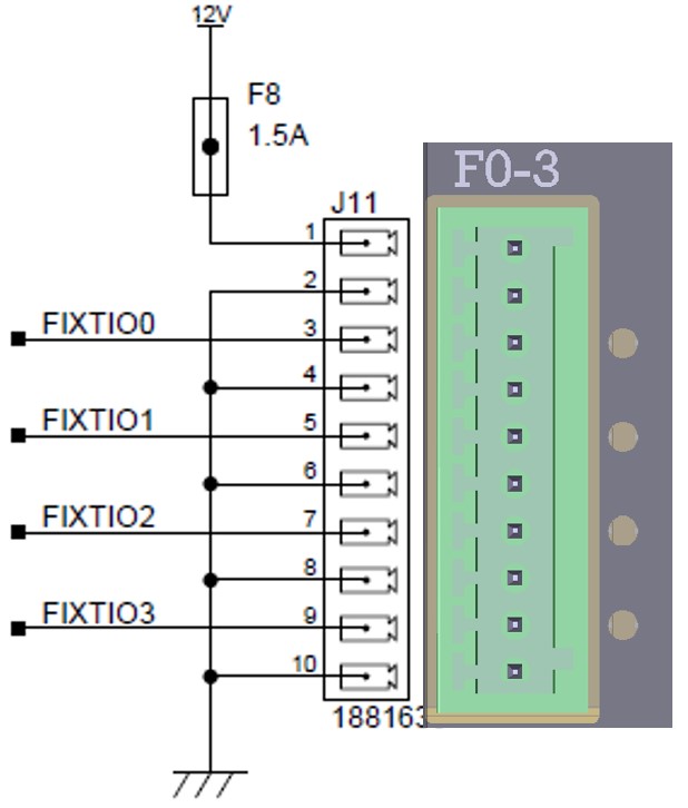
Figure 2 Fixture I/O

Fixture I/O frontend

The picture below shows the fixture I/O frontend. The input and the output are available at the same time for each fixture I/O. The output is of open drain type.

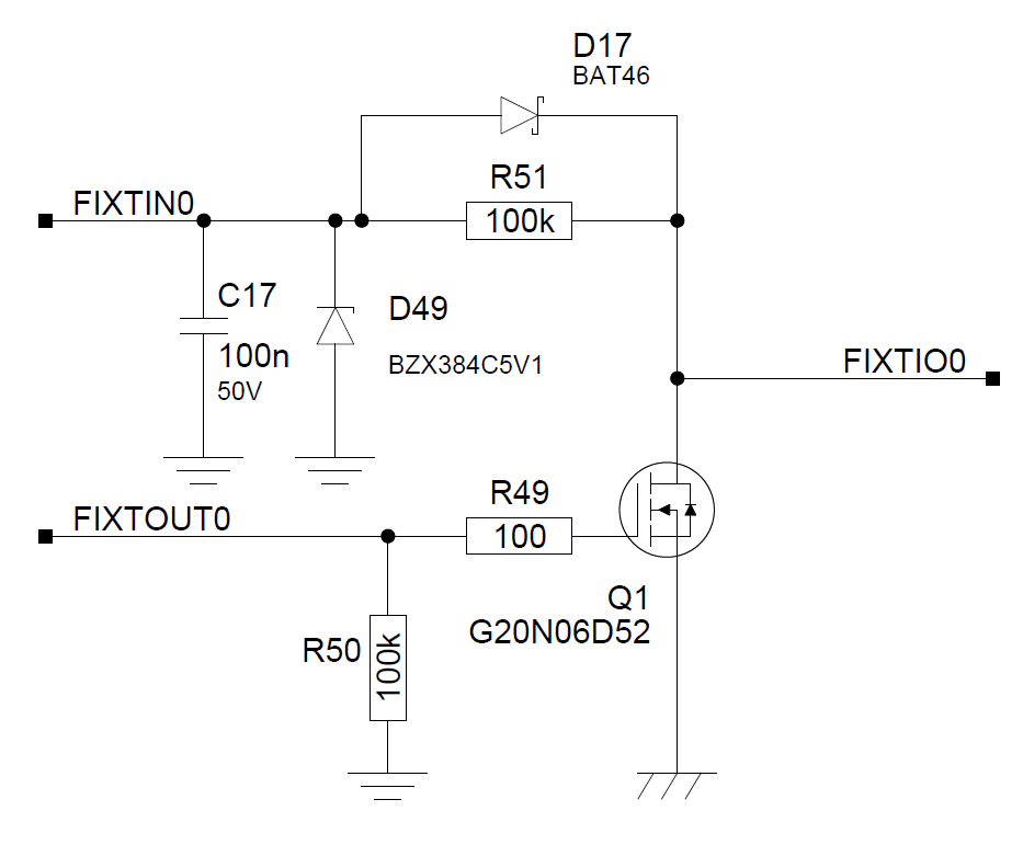
In the AGENT UI, both the fixture input channel and the fixture output channels are displayed.

If the fixture I/O should be used as an input, keep the FIXTOUT = FALSE and read the FIXTIN channel. Conversely, when used as an output, alter the FIXTOUT between TRUE or FALSE. When it is set to TRUE, the output will be asserted (grounded).

Having the fixture input available in conjunction with the fixture output has an additional benefit, as you can use the fixture input to verify the correct state, thus monitoring the behavior.

Fan connector

The fan connectors (5) is constituted by two 5V fan controllers. Fan connector pinout:

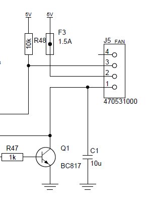
Pin 3 = TACHO input
Pin 2 = 5V Supply
Pin 1 = PWM

Note that when controlling the fan from AGENT UI, the control output is default disabled. In order to enable it, you have to click the checkbox next to the channel.

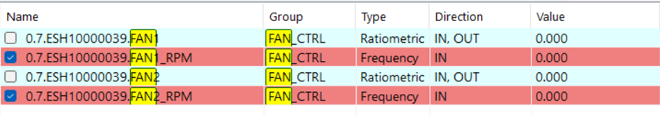
The fan speed is controlled ratiometric with a value between 0-1 where 1 = 100% speed.

The RPM of the fan is measured by the FANx_RPM channel. Note that the RPM assumes a 2-pole fan and might not be accurate.

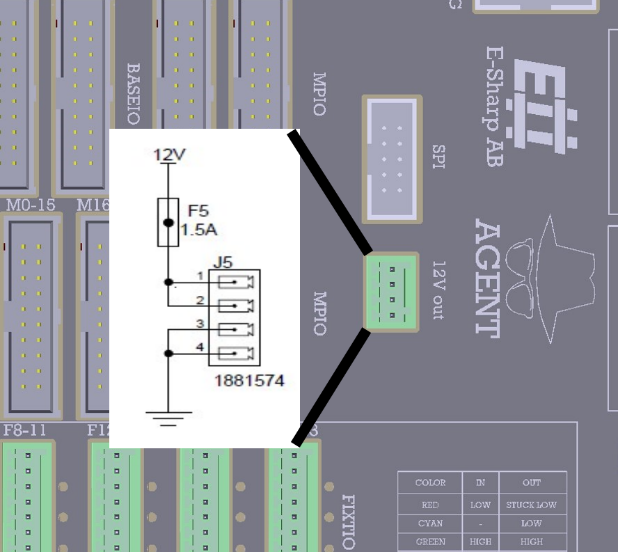
12V

There is one 12V connector on the AGENT. Pin 1 and 2 is 12V. Pin 3 and 4 is ground.

I2C Connectors

The two I2C connectors are based on P82B715, which means that it has to have a similar receiver on the other end of the cable.

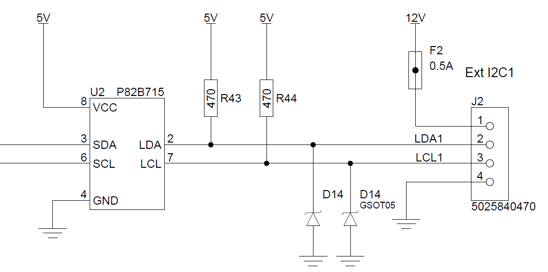
The connector type is a Molex 5025840470, mates with Molex 5025780400.

UART Connector

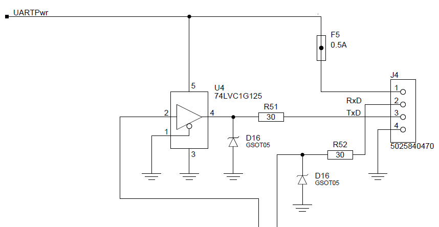
The connector type is a Molex 5025840470, mates with Molex 5025780400.

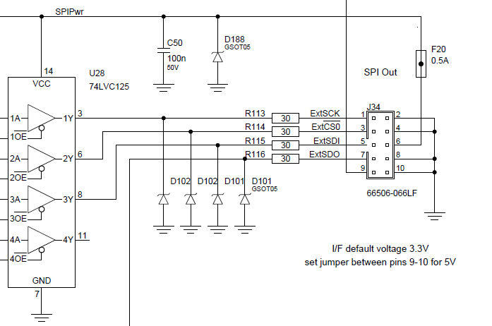
SPI Connector

JTAG Connector

Currently unused.

AGENT™ specifications

AGENT comes with a default set of modules and functionality. The modules can be replaced to adapt AGENT to the need of each customer.

Accordion Modules

The Accordion™ build system offer a wide range of different modules that allow you to customize your test solution or be plugged into your AGENT™ system directly.

AGENT™

The base unit comes with fixture control, I2C/UART/SPI/JTAG connectors. 5 module slots + 2 expansion slots.

AGENT

AGENT™ specification table

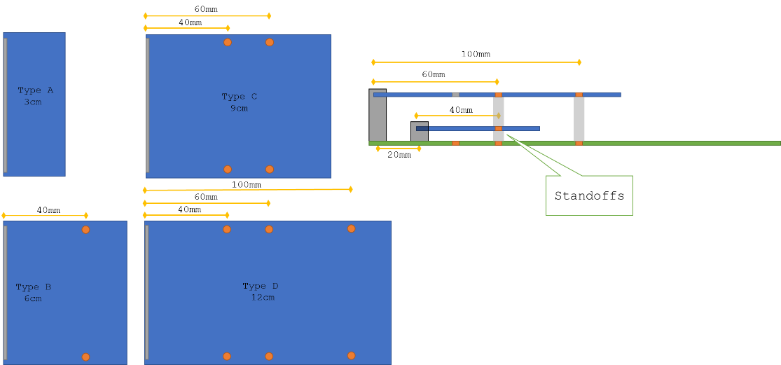
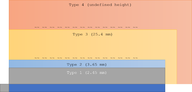
Module sizes

MPIO Module (SPI based)

ESH10000004

64 channel multi-purpose input/output module. Each channel can be individually configured to be either analog input/output or digital input/output. It can also measure resistance on channels 1-56.

Multi-Purpose I/O module (SPI based)

MPIO Specification table

5V tolerable. Voltage translation and protection must be done externally depending on the application.

Approximate sample times (excluding channel setup)

Note that the sample times are not guaranteed and are affected by service- and maintenance procedure calls from external application as well as network latency.

MPIO Module (I2C based)

96 channel multi-purpose input/output module. Each channel can be individually configured to be either analog input/output or digital input/output.

Multi-Purpose I/O module (I2C)

MPIO Specification table

5V tolerable. Voltage translation and protection must be done externally depending on the application.

Approximate sample times (excluding channel setup)

Note that the sample times are not guaranteed and is affected by service- and maintenance procedure calls from external application as well as network latency.

GPIO Module

96-channel general purpose digital input/outputs, push-pull or open drain, configurable I/O voltage per bank. 6 banks, 16 channels each.

General Purpose I/O module

GPIO Specification table

+/- 10mA drive capability per I/O

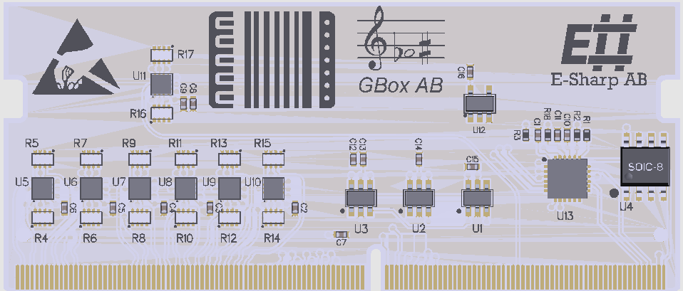
DUT Module

ESH10000010

Lab/Prototype board that allows for easy access to signals through 2.54mm headers. It also includes headers for 8 channels I2C, SPI and UART

Device Under Test interface module

8 channels I2C multiplexer. SPI/UART/JTAG buffers on-board.

Thermocouple Module

ESH10000008

40 channels, 2-, 3- or 4-Wire RTDs, Thermocouples, Thermistors and Diodes. Detection of faulty sensors and built-in automatic cold-junction compensation.

Thermocouple module

Thermocouple standards: B, E, J, K, N, S, R, T, temperature range between -265˚C to over 1800˚C

2-, 3-, 4- wire RTDs, thermistors and diodes.

6x 24 bit ∑∆ ADCs gives 0.1˚C accuracy

Thermocouple specification table

Analog Multiplexer Module

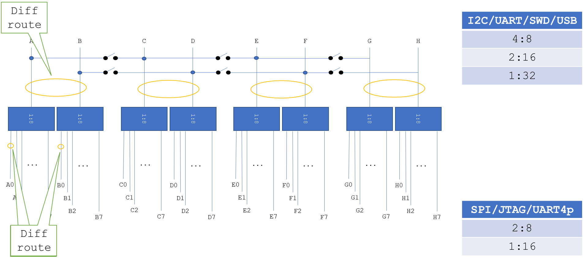
10*8 Multiplexer configurable as 1:80, 2:40 …10*8. Lanes A-B, C-D … J-K are length matched.

Option to route Accordion’s SPI, I2C and UART buses to all channels.

Analog Multiplexer module

90Ω impedance. Pairs are length matched with an impedance of 90Ω. Mount option to remove stubs in case Accordion SPI/UART is not needed.

Analog Multiplexer specification table

The picture below shows the internal structure of the multiplexer module. On the common side, up to 10 channels can be used individually multiplexed out to 8 channels each (8x10).

Note that the multiplexers are analog and bidirectional, which allows demultiplexing operations as well.

Possible multiplexer options

For 2-pin buses such as I2C, UART (RX/TX), SWD and USB, the following configurations are possible:

#Sources #Destinations #Total buses

4 10 40

2 20 40

1 40 40

For 4-pin buses such as SPI, JTAG, UART (RX/TX/CTS/RTS), the following configurations are possible:

#Sources #Destinations #Total buses

2 10 20

1 20 20

VOUT Module

24 Channel linear power supply that operates in 2-quadrants (able to both sink and source current).

VOUT module

Internal (5V) or external power supply

Range: 0-5V or 0-12V (external supply), up to 400mA per channel. For higher output solutions, a heat sink can be mounted.

RF Switch Module

36-Channel RF switch module 0.1 to 6.0 GHz switch designed to be used as a compact RF switch for galvanic or sniffer antenna applications.

RF Switch module

PSU Expansion module

Dual-channel, 2-quadrant power supply module with voltage/current measurements and sense.

PSU Expansion module

PSU Expansion module specification table

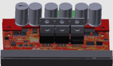
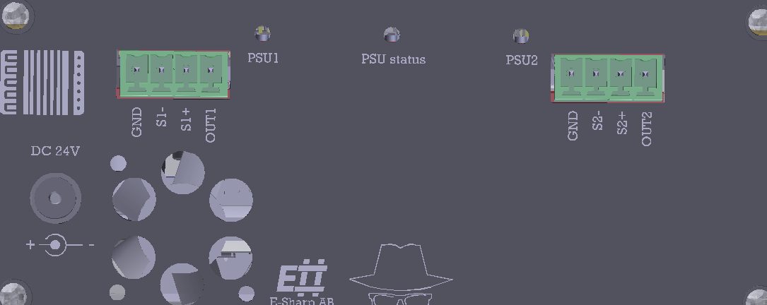
Picture of side panel when PSU module is installed. The connector is: Phoenix 1803293, mates with for example Phoenix 1803594 (other mating options exists).

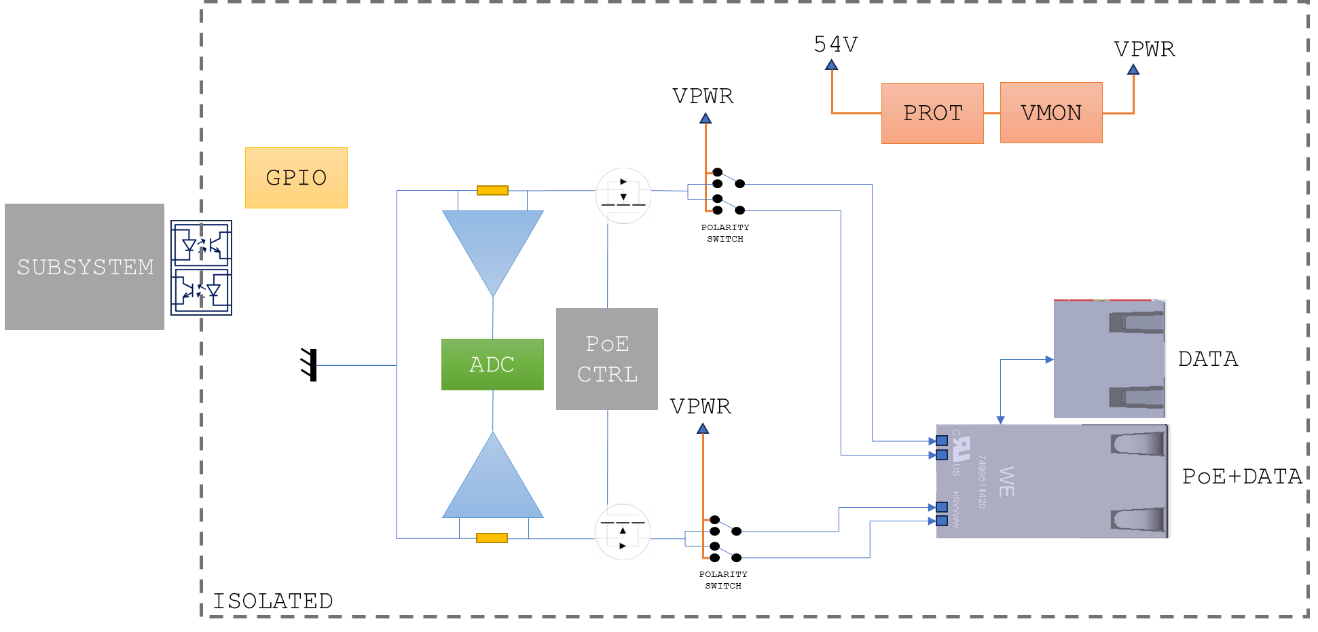
PoE Test Adapter module

802.3bt capable of class 8, 90W. Isolated with polarity switch, voltage and current measurements.

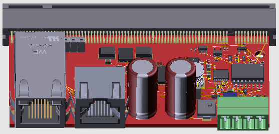
PoE Test Adapter Expansion module

PoE Test Adapter module specification table

Accordion Controller

Install from : https://esharp-accordioncontroller.s3.eu-north-1.amazonaws.com/setup.exe

The software implementation for Accordion AGENT™ is divided into two parts; On part resides on the AGENT™ itself, the other part is communicating with the system through a MQTT API.

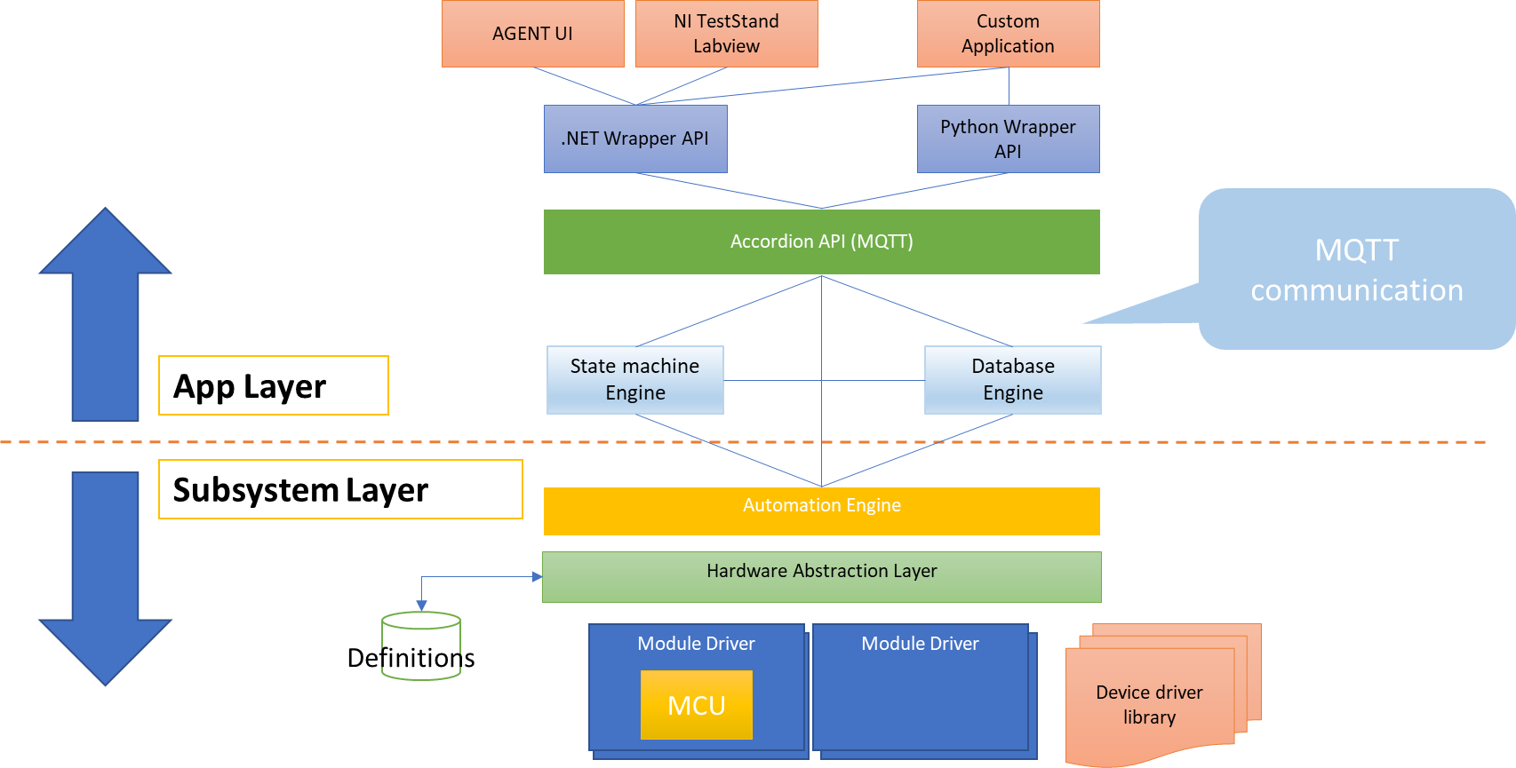
Figure 3 AGENT layers

On the application layer, a MQTT wrapper provides access to the AGENT hardware.

The automation handler goes through a hardware abstraction layer (HAL), which abstracts the actual implementation of the drivers for each Accordion module.

The ‘Channel’ concept

All functions in an Accordion system are abstracted through a ‘Channel’ concept. A channel could be anything from a Digital or analog input or output, a temperature input, a register, or a communications channel. The intention of this abstraction is to provide an intuitive interface towards complex functions.

When the Accordion system boots, a discovery process is started to find all attached hardware modules. Each module reports the channels it supports.

The ‘value’ of a channel is always represented as a string. If it is a boolean-type value (as for a digital channel), the string value is either “true” or “false”. For floating point numbers (as for an analog channel), the string value is always a value convertible from a double value with dot as a decimal separator “1.234”.

Values are always in SI units if applicable. Measuring a voltage returns the value in ‘Volts’ for example. Temperature returns the value in °C.

Channel definitions

The following channels are defined:

Analog

An analog channel can either be an input or an output. Gain and Offset settings affect how the value is converted in the form y=kx + m, where k = Gain and m = Offset.

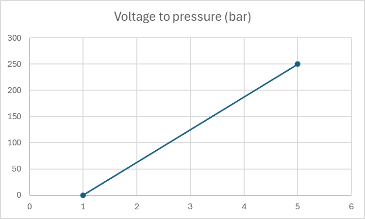
For sensors (input) or excitation networks (output) this can be very useful when working with linear systems. Say for example that you use a pressure sensor that measures the pressure in bars where 1V equals 0 bar and 5V equals 250 bar. Setting Offset = 0.5 and Gain = 62.5 gives the resulting value directly in bar’s instead of having to convert the value by hand.

When an analog signal is an output, the reversed calculation is made. This means that for a Gain of 2, it is assumed that some external amplifier doubles the signal, hence the output value from channel is halved. External attenuator can be modeled in the same way by using, for example Gain=0.5.

Digital

A digital channel can either be an input or an output. Depending on the capabilities of the module that provides the channel, it could have a configurable PushType (OpenDrain, PushPull) or a configurable PullType (None,Up, Down) depending on if it is configured as an output or an input. A digital output configured with OpenDrain means that the digital state ‘true’ will short the output to ground, and ‘false’ will render the output to be high impedance (High-Z). A digital output configured with PushPull means that the digital state ‘true’ will push the voltage up to the IO Voltage, and ‘false’ will pull the voltage down to ground.

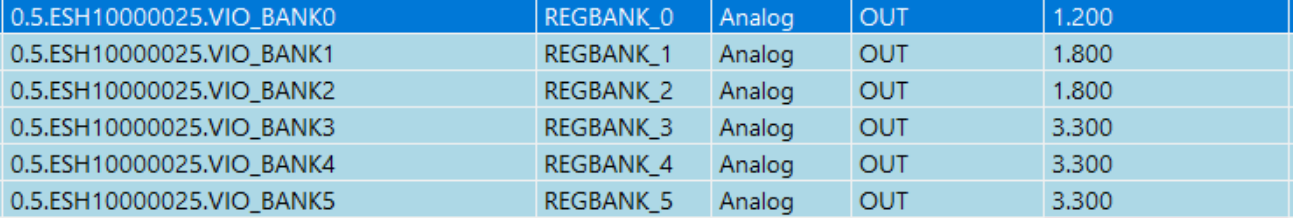
For the IO Voltage setting (if supported), it sets the IO voltage that is used with the PushPull configuration. Note that for the GPIO module (ESH10000025), the IO Voltage can’t be configured per-pin but rather per-bank (groups of 16 GPIOs) and is then controlled by another channel called ‘VIO_BANKx

When a digital pin is configured as an input, the PullType sets if there should be a pull-up resistor, a pull-down resistor or no resistor. If a pull-up resistor is selected, it is weakly pulled up to the IO Voltage. A pull-down resistor is a weak resistor down to ground. The exact resistance of these pull resistors is not defined but in the range of 100kΩ.

Multiplexer

A multiplexer channel is seen as representing the common node of a multiplexer of arbitrary size and its value represents the currently selected wiper node. The multiplexer is enabled or disabled using the channel’s Enabled property.

Temperature

The temperature channel is typically an input that measures a real-world temperature and returns the value in °C. Most temperature channels are not configurable, but for example the Thermocouple module (ESH10000008) can configure what type of sensor that is attached. The possible values for the SensorType are:

(Entries in gray are not directly supported, contact E# for more information if this is needed.)

For thermocouples, a reference cold junction must be provided, which is done with the field ‘Coldjunctiondestination’. Possible values are ‘CH<id>’ where <id> is [00 to 20] and denotes what channel that should provide cold junction measurements. Several or all thermocouple channels can be associated with the same cold junction channel.

A cold junction channel can’t in it self be a thermocouple channel, it has to be a sensor that accurately converts real-world temperature’s, such as a diode or RTD.

Resistance

A Resistance channel typically measures resistance. Resistance is measured indirectly by applying a known voltage over the load, measuring the current that flows in the circuit and by that calculate the resistance using ohms law.

Counter

A Counter channel counts pulses. To reset the counter, the channel could be disabled and re-enabled.

Frequency

A Frequency channel could either be an input or an output (i.e. measure or generate a frequency).

Actuator

An actuator channel is similar to a Digital output channel but has the additional capability of toggling the signal with a specific interval. If the ‘ToggleEnabled’ field is set to ‘true’, the channel will toggle back into its default value after ‘ToggleTimeMilliSeconds’ has elapsed.

PowerSupply

A PowerSupply channel is used by a Power supply to configure its output. Enabling/disabling the channel corresponds to turning the power supply output on/off. The value of the channel sets the output voltage expressed in volts.

‘CurrentLimit’ sets the current limit (if supported) of the power supply and ‘OverCurrentResponse’ sets how the power supply should react if the ‘CurrentLimit’ is reached. ‘OverCurrentResponse’ can either be ‘Off’ (turn off power supply output) or ‘Limit’ (enter constant-current mode).

Register

A Register channel is a channel type that handles all other aspects that is not covered by the other channel types. A typical case for a Register channel usage is exposed chip registers (byte-oriented) or string-based values that can be set or read.

Ratiometric

A ratiometric channel is used for a value that is relative (ratiometric) to another property. The value is typically between 0-1 (0-100%). An example is fan setting, where the fan is regulated between 0-100% of its capacity.

UART/SPI/I2C

These channels are specific to bus communication and can’t be read or set directly but rather from the ‘Bus Communication’ tab page.

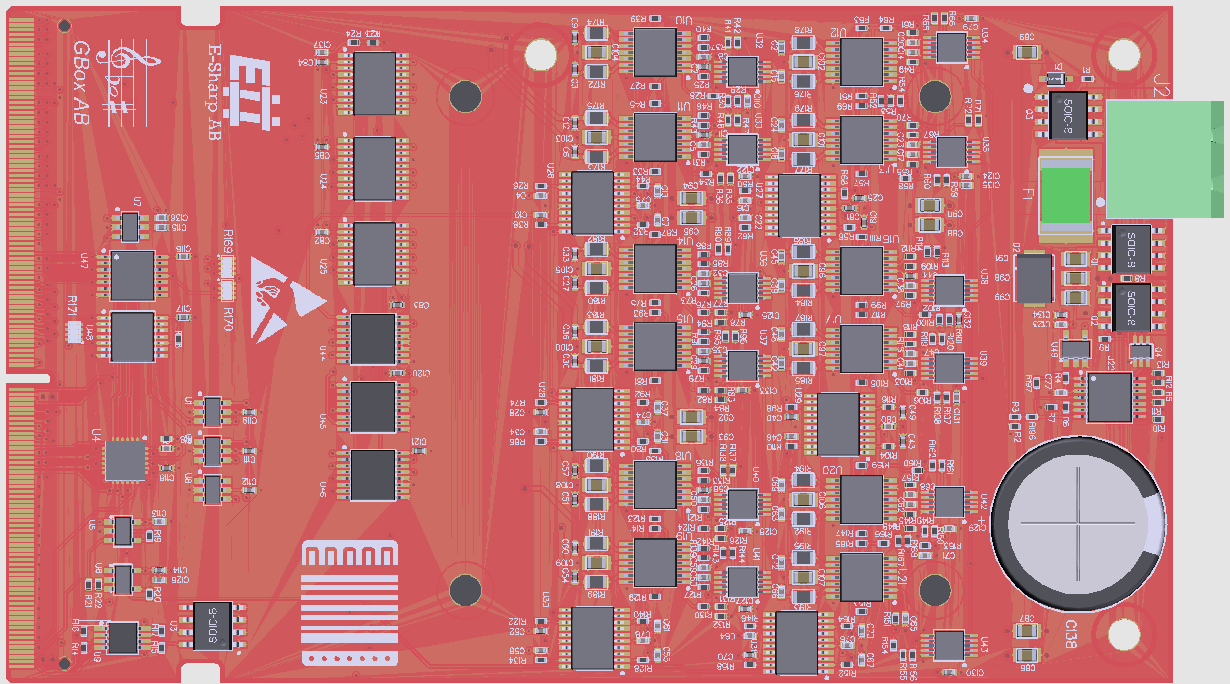
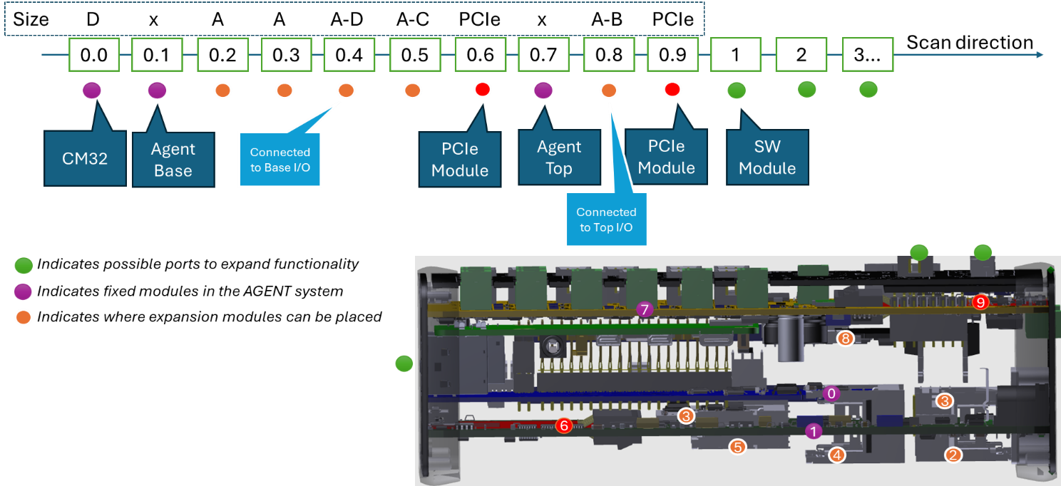
Module slots and channel resolving

When the Accordion subsystem boots up, all module slots are queried, and the installed modules will trigger loading of specific module drivers.

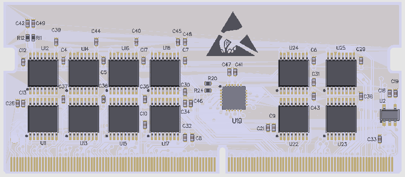
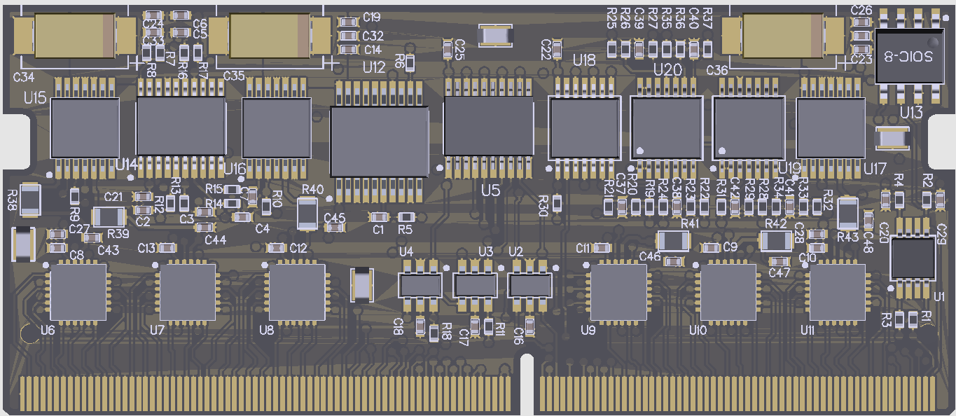
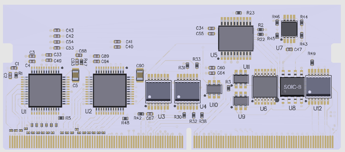
The picture below shows the order and position of modules and the respective size of the modules that can be placed there.

Software Modules

Software modules are additional functionality that can be loaded into the Accordion framework and act as any other (hardware) module in the system. This can be very useful, as new peripheral features and functionalities can be integrated into the same software/driver structure.

A software module must be pre-configured in the HW configuration.

Loading of a software module can be done in two ways, either upon boot by configuring the module to auto-start or by loading the module dynamically by using the Engine.LoadModule channel.

The Accordion subsystem provides the following channels for working with software modules:

Alias translation file

An alias translation file is used to provide naming and configuration to the channels.

Loading an alias translation file has two purposes; First it makes programming much easier as the hardware has understandable and descriptive names. Second, it also configures an initial state and checks that all the defined hardware responds as expected. Many channels can be configured in different ways, such as either as an input or an output.

Connecting

Enter the host name in the form <serial number>.local (“.local” is not strictly necessary, but might shorten the connection time). The serial number can be found on a sticker on the product.

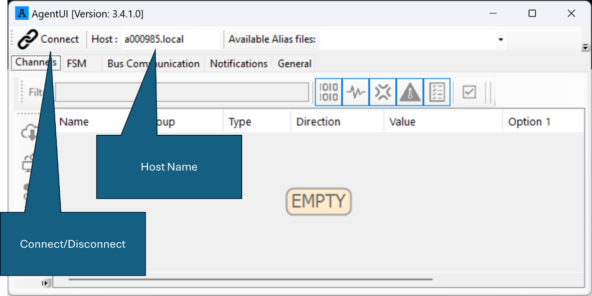
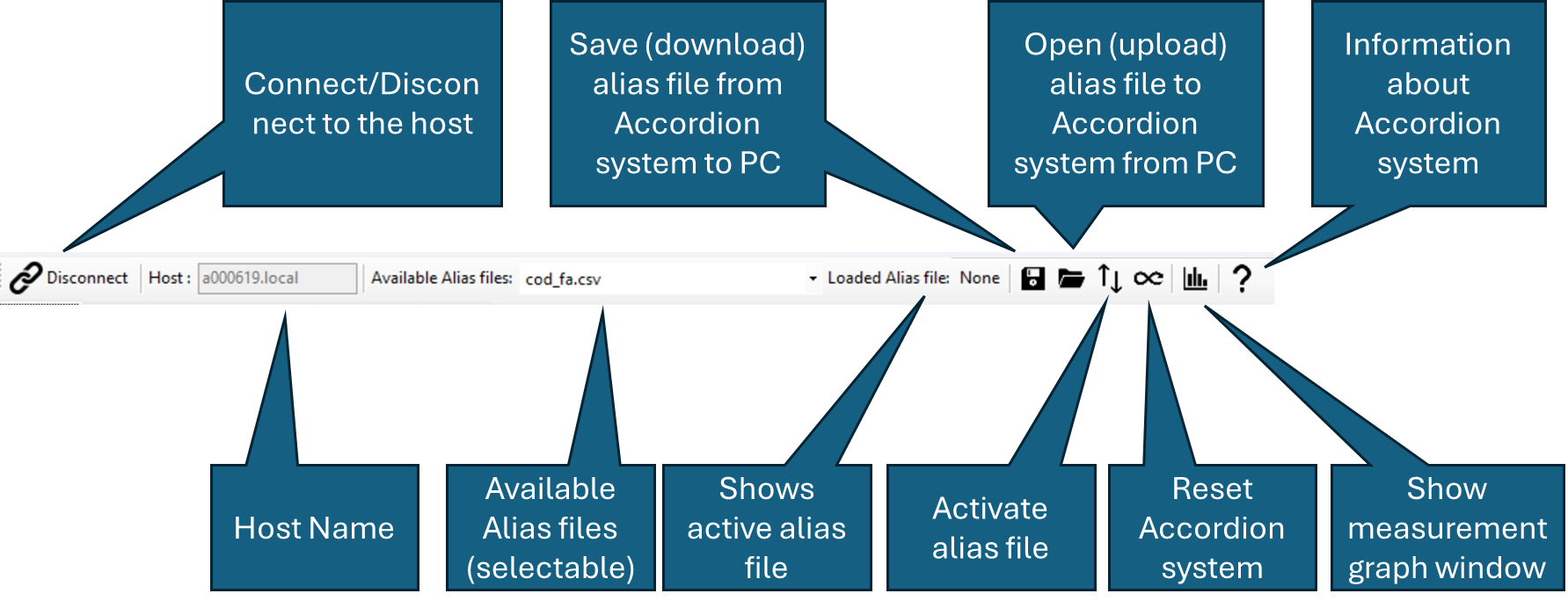
Main menu

Configuration

Tab page ‘Process Config’

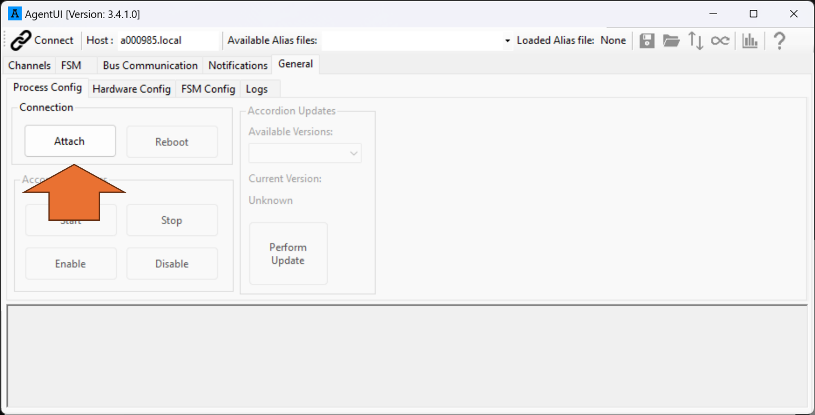
Go to the tab page “General” and press ‘Attach’

Note that you don’t have to connect using the ‘Connect’ button prior to this. All functionality on the ‘General’ tab page uses another communication mechanism (SSH/SCP) and is not related to the MQTT connection.

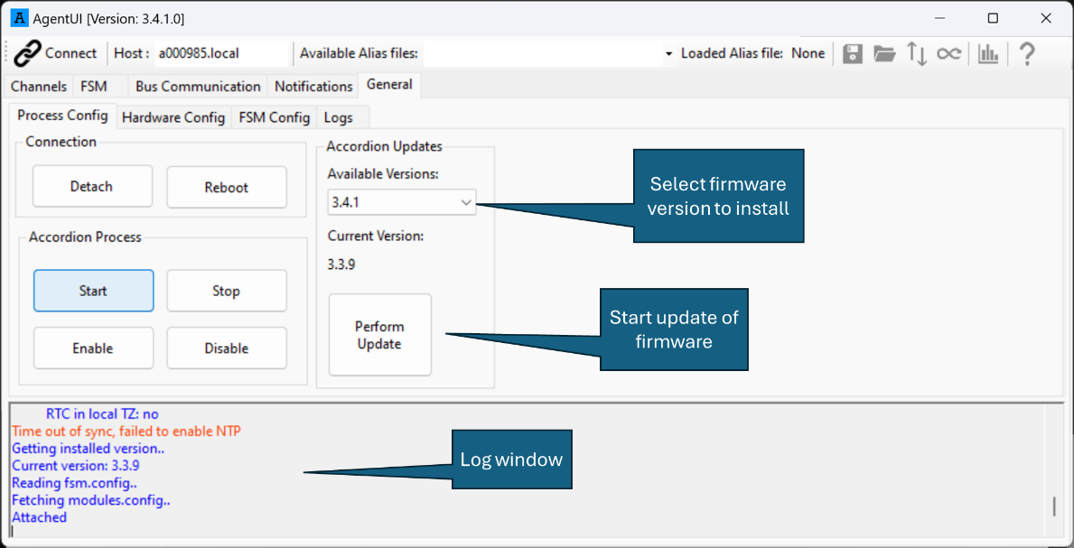
Once attached, you can configure things related to the Accordion firmware on the embedded linux PC, such as changing firmware.

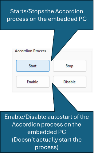
The Accordion process group is used to start or stop the Accordion process on the embedded linux PC. Stopping and starting the Accordion process here is equivalent to powering off/on the system.

It is also possible to set if the Accordion process is auto started when the unit powers up or not by setting Enable/Disable accordingly.

Tab page ‘Hardware Config’

On this tab page, the software modules can be configured. Software modules are external implementations that allow peripheral functions to integrate into the Accordion framework.

The module to configure is selected in the drop-down menu.

Add – Add a new entry

Remove – Remove selected entry

READ – Read entry’s settings

WRITE – Write entry’s settings

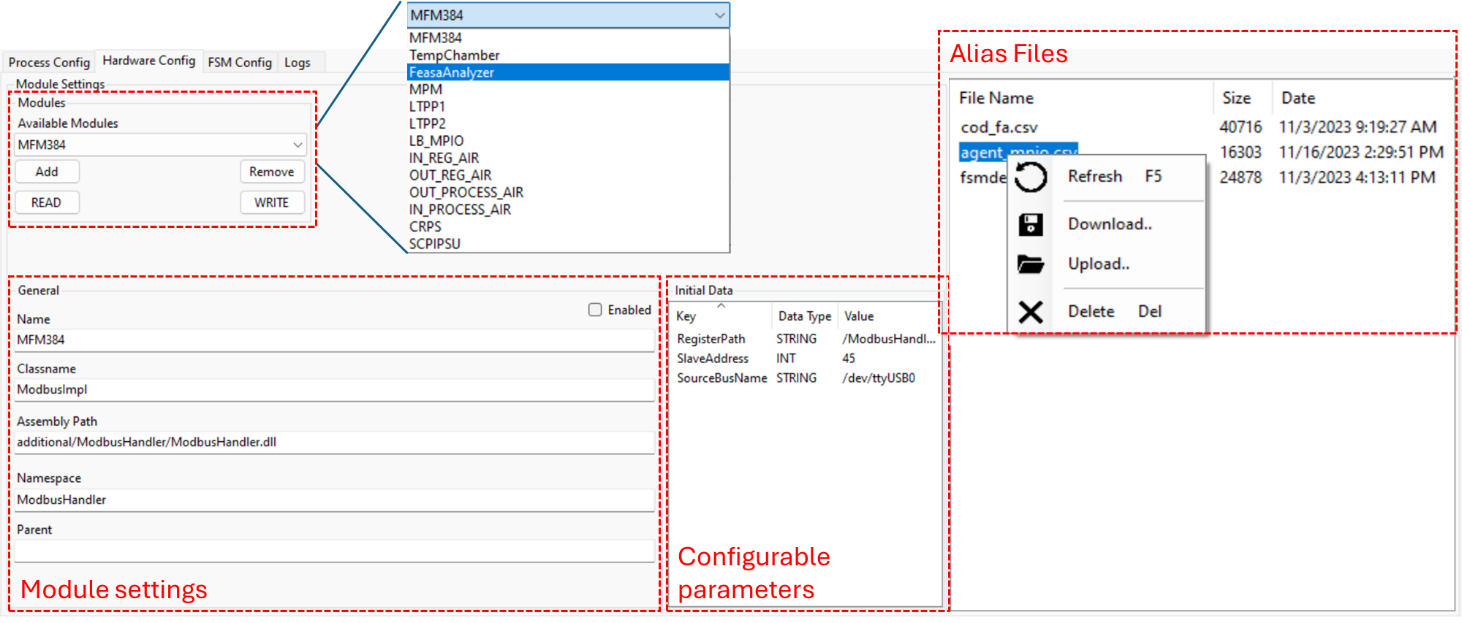
In the ‘Module settings’, class information is configured. This needs to match the software module’s specific properties and shouldn’t be changed. The ‘Enabled’ checkbox sets if the module should auto-load upon startup.

In the ‘Configurable parameters’, any initial data that is used by the module can be entered. Refer to the developer of the specific module for details.

In the ‘Alias files’, alias files can be up-/downloaded. Note that alias files can also be up-/downloaded in the main menu.

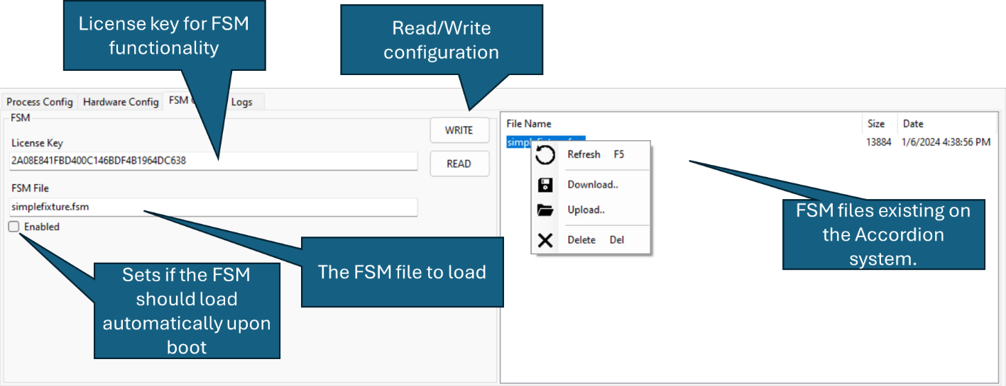
Tab page ‘FSM Config’ (Finite State Machine Config)

On this tab page, the FSM is configured.

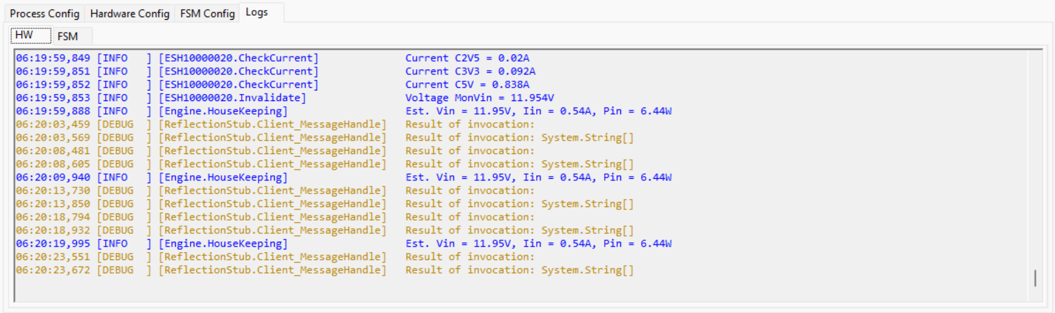
Tab page ‘Logs’

On this tab page, the raw logs from the Accordion Processes are showed. The ‘HW’ tab page shows logging from the hardware process whereas the ‘FSM’ tab page shows logging from the State machine engine process.

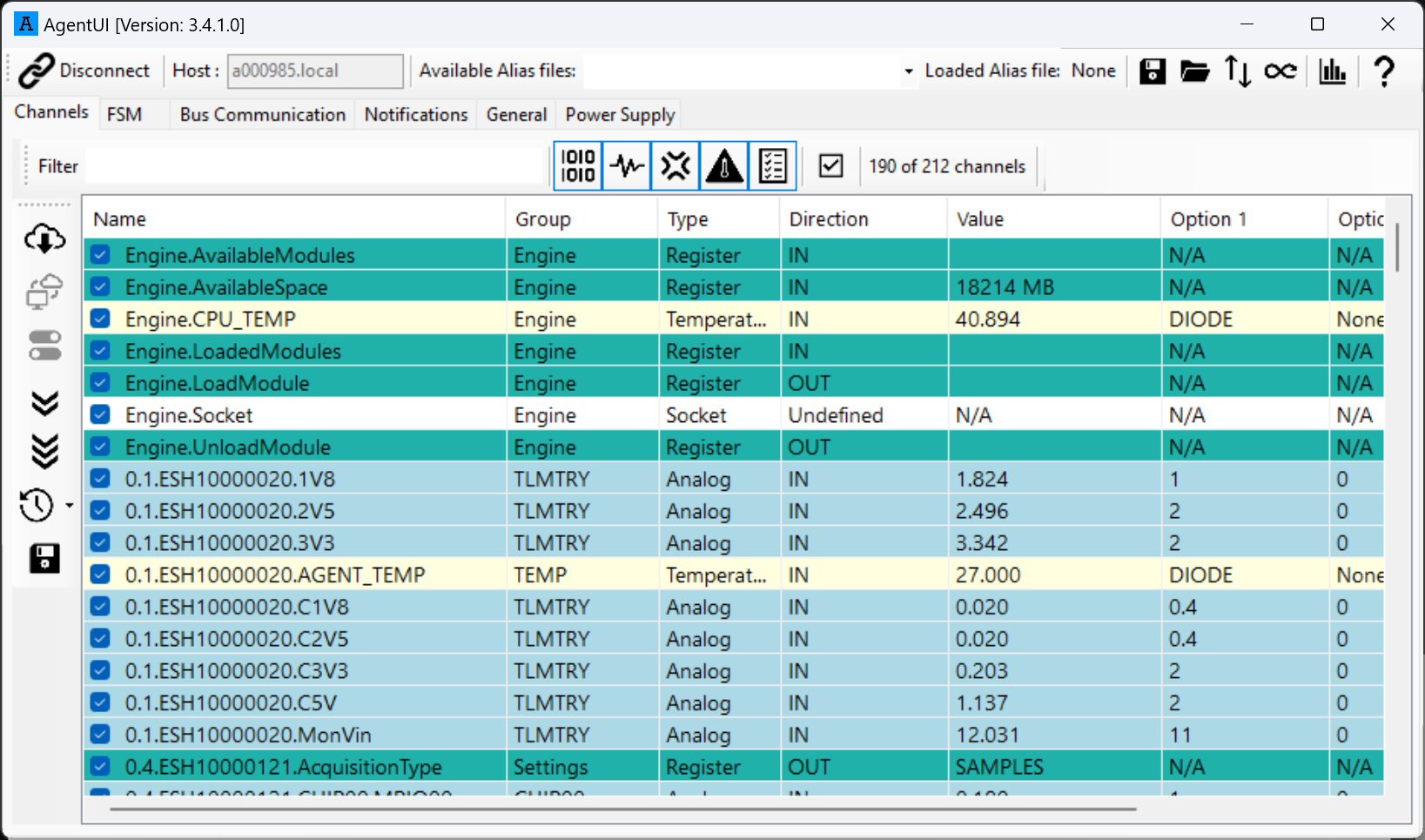
Channels

The ‘Channels’ tab page displays all available channels on the attached system.

Menus

Appendix 1: SME Option

Introduction

The State Machine Engine (SME) option in Accordion™ is a powerful autonomous state machine engine that runs unsupervised on any Accordion™ product. This feature is useful when controlling a machine or a fixture as it provides autonomous behavior without a host computer controlling it and it offloads the host computer many or all the tasks associated with controlling a machine.

State machine basics

A state machine (or finite state machine to be precise) is an abstract machine that can be in exactly one state of a finite number of states at any given time.

The state machine can change from one state to another based on an input value. An input value that causes a transition is called a trigger. A change between states is called a transition. Upon entering a state, zero or more actions could take place, for example setting a value, starting a PID regulator, starting or stopping timers.

It is worth noting that a transition is immediate. This is inherent from the way a state machine functions – it is always in exactly one state at any given time. It might be tempting to think that “something happens” during the transition but it doesn’t.

A typical example would be that a state action sets a digital signal that actuates a cylinder and you want to reach a destination state when the cylinder arrives to its destination. In this case, you need a transitional state that sets the actuator and starts a timer for waiting for it to arrive (see example below)

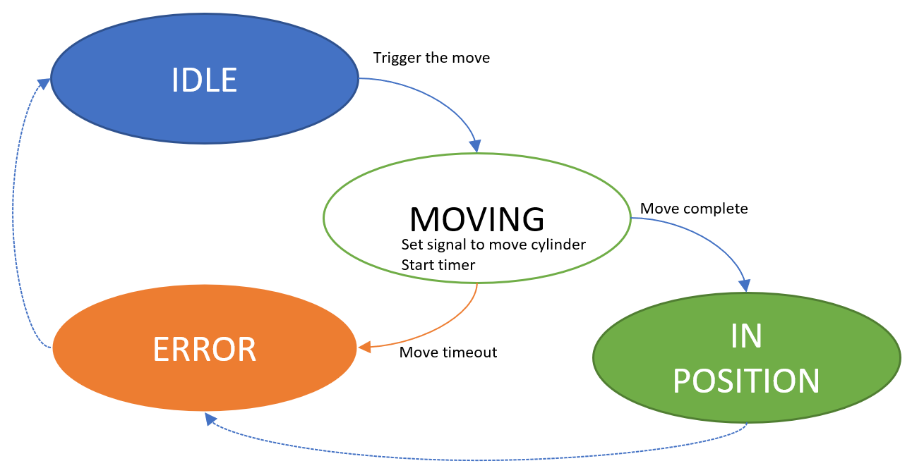
From a starting state (IDLE), something happens that triggers a move request of the cylinder. The state machine transitions to the MOVING state, which sets the signal to move the cylinder. It also starts a timer to prevent getting stuck in this state forever in case the arrival signal never comes. The state machine will be in this state until the arrival signal is asserted (goes to IN POSITION) or the timeout elapses (goes to ERROR).

See Wikipedia for more information.

The state machine engine in Accordion™

The Accordion™ subsystem is running on the Accordion hardware, which communicated via MQTT broker that serves streaming messages from the running state machines.

The SME runs in an isolated thread and communicates through the subsystem towards either a host computer or the hardware modules on the Accordion.

The hardware subsystem is also isolated and runs the hardware engine through an abstraction layer.

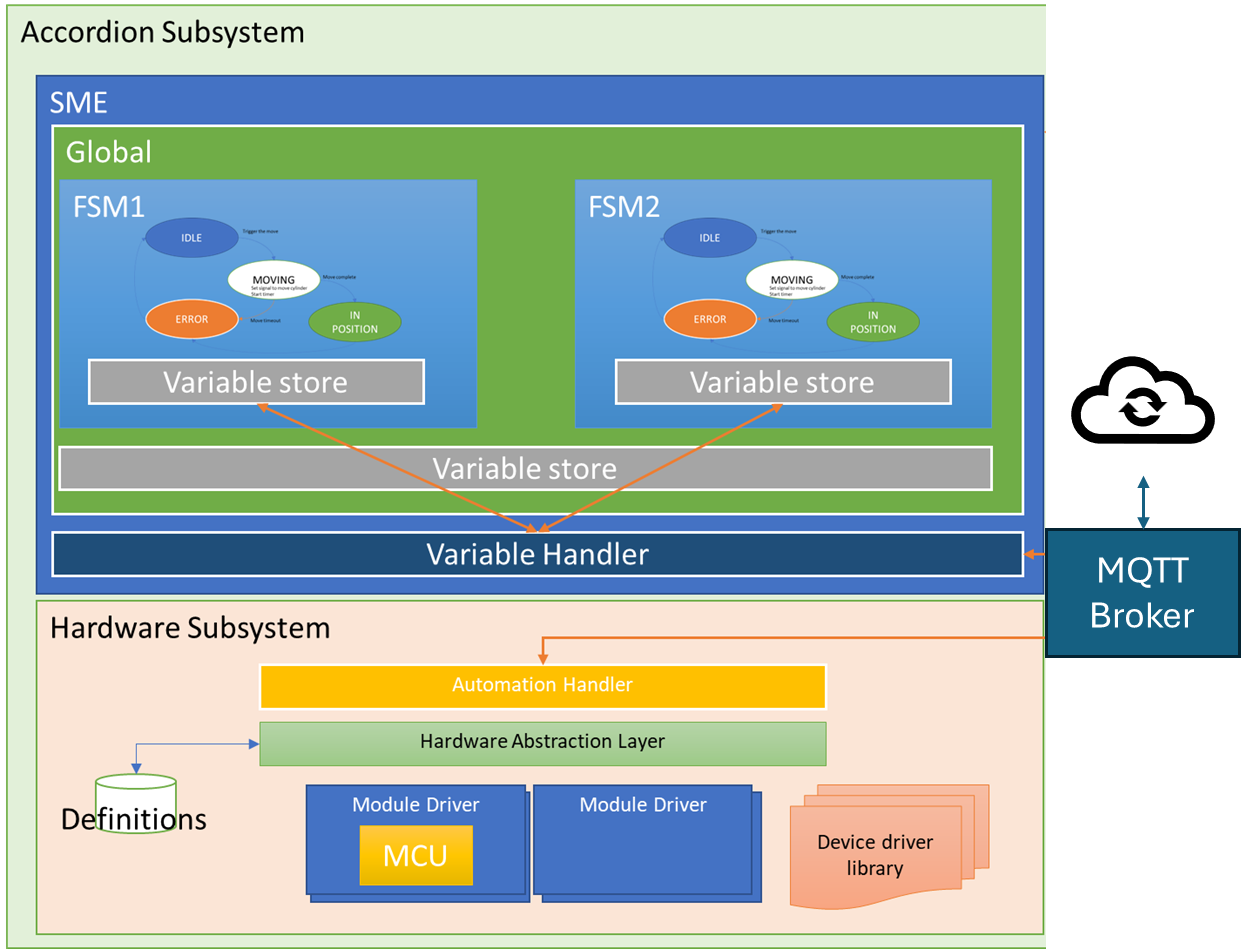
The SME could run one or several state machines in parallel. The SME treats all defined state machines as independent of each other and they are executed asynchronous in separate threads.

Each state machine has a name (Context) and a minimum configuration requires at least two states; One state marked as Initial and one additional state, as each state requires a trigger to another state. The SME implementation in Accordion™ doesn’t support triggers to the same state that fires it.

They can share common variables, most notably the HardwareSignalVariable’s, which are defined in the global context. The global context is special, as it is the parent of all state machines and provides a variable store also for inter-state machine communication.

Getting started

Assuming the SME option is installed on your Accordion™, you can select if the state machine should start automatically upon boot or not. This behavior is configurable by editing the setting found under “General->HW Config”. See AGENT Manual for more information.

Creating a state machine definition file

Open the example project in Visual Studio and run it. This will produce a valid state machine file that can be viewed in AGENTUI™ and uploaded to your Accordion™.

Note that the file produced is not human readable, as it is in binary format.

The state machine project is automatically checked for warnings and errors. Carefully examine any errors that the validator emits; the messages are useful for creating a well-formed state machine.

Variables

Everything in the state machine revolves around variables. It is variables that receives measured values, sets the hardware to a certain state, triggers transitions and so on. The Accordion™ SME introduces a powerful variable handling and detailed knowledge of how the variable engine works is key to a successful implementation of a state machine.

All variables, regardless of type share some common treats:

• They have a owner (a variable is defined either in a Global context or in a FSM definition)

• They have a unique name (referred to as ‘key’)

• They have a value type (for example boolean, string, int, double)

• They might have a description

• They might have a default value

• They have a sample depth setting (i.e. how many samples are stored)

• They have a numeric operation setting (Average, Min, Max, Diff, MaxHold, MinHold)

• They have a UsedExternally flag, which omits the variable from warnings of unused variables

• They have a Value property, which returns the calculated value of the variable based on type, sample depth and numeric operation setting.

Most of the variables (except VirtualVariable and TimeoutVariable) have one or more underlying variable keys, as they typically operates on basis of another variable. For example, a LimitVariable contains a limit value and a key to another variable that the limit should be applied on.

A variable that is used in a trigger must be of type Boolean. This is a restriction imposed because a state transition must be deterministic. Let’s say a state transition should occur if a decimal number is higher than 5.35;

• The variable receiving the number 5.35 could for example be a pressure sensor that the hardware measures (a HardwareSignalVariable of type double)

• Then you would create a LimitVariable where the limit value is 5.35, and the LimitType is Greater

• The trigger points to the LimitVariable, which turns true upon that the HardwareSignalVariable surpasses the limit 5.35

• The trigger fires and the state changes to the destination state.

There’s no limit on how large the hierarchy of variables can be. There are no restrictions of how many dependent variables you can have. In practice, this means that a single variable can be the source for an arbitrary number of other variables.

The defined variable types are:

For each defined variable, a dependency tree is built by the state machine engine. If any variable changes value, all dependent variables are updated as well. The operation recurses up the dependency tree until all dependent variables are updated. Note that the validation engine will prevent you from adding circular dependencies as this would cause a stack overflow condition during runtime.

HardwareSignalVariable

A HardwareSignalVariable is used as a backing variable towards the Accordion™ hardware engine. All HardwareSignalVariable’s must be added to the Global context as they per definition doesn’t belong to any specific state machine. Adding such signal to a state machine context will throw an error.

The name (key) of a HardwareSignalVariable must be identical to a signal name defined in the alias translation file that resides on the Accordion™ system.

A HardwareSignalVariable also have two important properties that controls how the Variable Handler will treat the variables; A direction and a hardware group name.

The direction setting tells the Variable Handler if it should read or write a value towards the hardware engine.

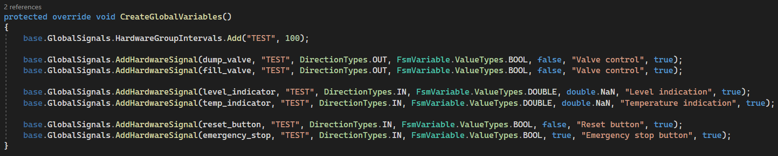
The hardware group name tells the Variable Handler which signals that belongs together and should be invalidated (handled) at the same time. This has an important performance aspect; many hardware signals are being read or written simultaneously regardless of whether all- or just one signal is requested. For example the fixture I/Os are all read in a sequence so all fixture I/O access from the state machine should be placed in the same hardware group name for optimum performance.

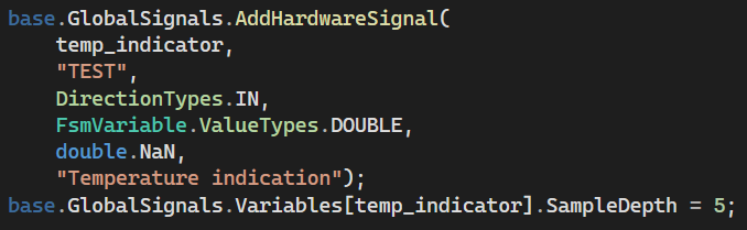
Trying to add a HardwareSignalVariable without first adding a HardwareGroup will throw an error. Each variable must be associated with a HardwareGroup. A HardwareGroup must have an interval associated with it (in the example below, the group “TEST” will be read each 100 ms).

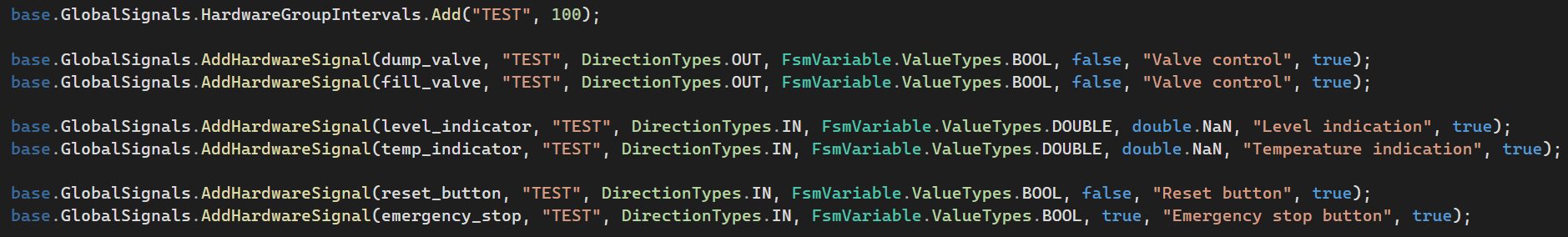
A state machine can’t force a hardware read, it will be done automatically in the background of the Variable Handler regardless if a state machine cares about a value or not.

Writing to a hardware signal is slightly different; still, a HardwareGroup is required (with an associated interval), but the interval is disregarded and the hardware signal will be written immediately. The interval property for Direction=OUT type signals exists for future optimization purposes.

Note that for performance reasons, you should always select the longest possible invalidation interval. Intervals < 10 ms will most likely perform worse than a longer interval due to the flood of hardware communication that it triggers.

Be wise when selecting the hardware group names. As the state machine engine doesn’t know anything about the hardware, it can’t optimize how signals are being read and this can have significant performance impact. This knowledge must be supplied by the implementor.

Let’s say you have a bunch of Fixture I/Os which all should be read with 100 ms interval. Then you place all of these signals in the same hardware group name. You also have some thermocouple signals which would be fine reading with an interval of 5 seconds, you should place them in another hardware group name with the desired interval.

LimitVariable

A LimitVariable is used to impose limits on other variables. It can be added to both the global context and a state machine context.

A LimitVariable is always associated with another variable, has a value type, a limit type and a limit.

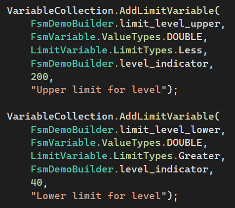
In the example above, two LimitVariable’s are added, both are applied to the same underlying variable (level_indicator), the first one sets that the value should be less than 200 and the second sets that the value should be greater than 40. When the underlying variable level_indicator is updated, also these two variables are updated and will resolve to either true or false, depending on the value.

The value of a LimitVariable is true if the underlying variable holds a value within limits and false if the limit is violated.

LutConversionVariable

A LutConversionVariable is used to convert a value from a source variable to another value using a supplied lookup table.

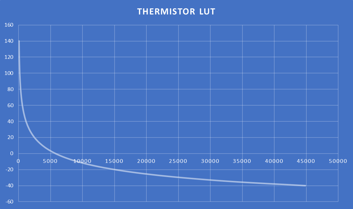
Let’s say you have a thermistor connected to a MPIO Module and you want to use the built-in resistance measurement capability to convert the thermistor resistance to a temperature.

In this case, you want to employ linear interpolation between the points in the lookup table.

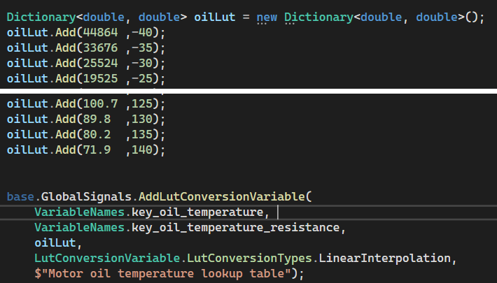
In this example, the LutConversionVariable itself is called key_oil_temperature, it will use the underlying variable key_oil_temperature_resistance which comes from the hardware subsystem and lookup that value in the first column and store an interpolated result that represents the temperature of the engine oil.

There are other situations where linear interpolation is not suitable, but where a step function works better. For example, we want to adjust the upper limit for a PID regulator depending on the measured temperature to make sure we have reasonable limits over the whole working range of the PID regulator. We have concluded that we want to use these limits:

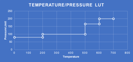
The snippet below shows how to add such a lookup table:

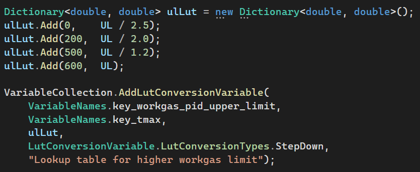
A LutConversionVariable can be configured to be either a LinearInterpolation type (showed in the first example), a StepDown type (showed in the second example) or a StepUp type. The StepUp type is similar to StepDown, but it selects the higher value rather than the lower in the defined intervals.

OffsetVariable

An OffsetVariable is used to offset a value from a source variable. In many cases, the relationship between two values are a better representation of what you are trying to control than the measured value itself.

Let’s say you have a value measured by the hardware (pressure-, temperature- or something else) and you want to know how much two values differ, an OffsetVariable can automatically calculate that value for you.

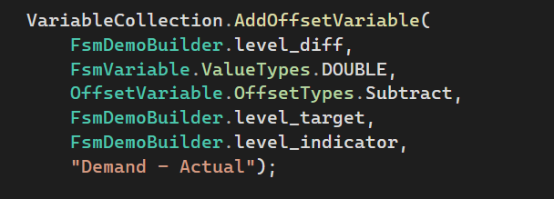
In the example above, we create a OffsetVariable level_diff, which takes the first parameter level_target and subtract it with level_indicator. The value produced is how far we are from our target value and we can use it to determine the appropriate action.

TimeoutVariable

A TimeoutVariable is used to allow the state machine to react to something after a specific time. It can be used for error checking as well as normal program logic.

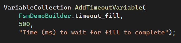
The example above creates a TimeoutVariable, with the name timeout_fill, the timeout value is 500 ms. Starting or stopping a TimeoutVariable is done in a state action using the commands StartTimer and StopTimer respectively.

VirtualBooleanVariable

A VirtualBooleanVariable is used to create an aggregated boolean representation of several other boolean values. There are many cases where combinatorial logic are useful, in particular when merging several status flags into one aggregated flag.

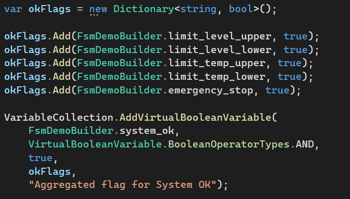
The example above creates a VirtualBooleanVariable with the name system_ok that will evaluate each variable and its state defined in the list of okFlags.

In adding the Dictionary<string, bool>, note that the first (key) argument is the variable name to examine, and the second argument (value) is the expected boolean value of that variable.

Note that all underlying variables must be of the type BOOL for a VirtualBooleanVariable to work. In this example, there are LimitVariable’s that are used to form a boolean result from a numerical value.

It is possible to configure a VirtualBooleanVariable logic to AND | OR.

Combining several VirtualBooleanVariable can create compound statements of AND/OR.

VirtualNumericVariable

A VirtualNumericVariable is used to create a calculated value of int/double values from several other int/double values. This is useful for example if you want to get the average, diff, min or max value from several temperature- or pressure sensors.

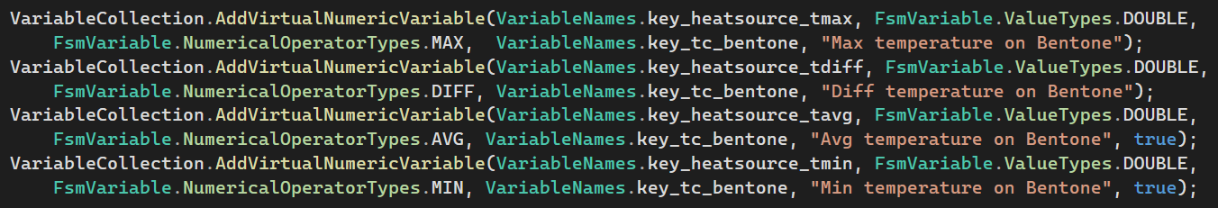
The example above takes an array of variable names key_tc_bentone which are connected to several temperature sensors and creates a new, aggregated VirtualNumericVariable for their MAX/DIFF/AVG/MIN values.

VirtualVariable

A VirtualVariable is a variable that has no underlying key, which can be used as the source value for other variables. As most variables require an underlying key, virtual variables are typically needed to serve values where there’s no HardwareSignalVariable involved.

Some of the use cases for a VirtualVariable are;

• As backing variables for a PID regulator

• Storing calculated results

• Use them as externally accessed variables that controls the flow (for example an external reset- or start signal)

A VirtualVariable can be of different value types, such as double/int/bool/string.

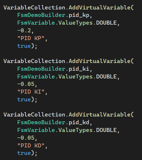
The example below creates the backing Kp, Ki and Kd variables for a PID regulator.

Building state machines

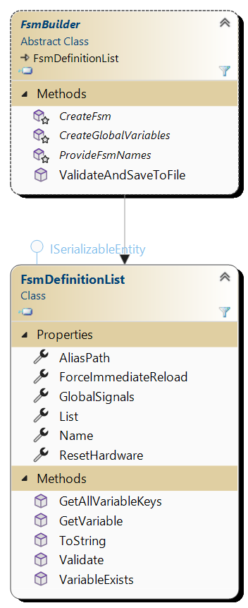
In order to simplify the process of building state machines, a few “Builder”-classes are available. You should implement a top-level class that inherits from FsmBuilder.

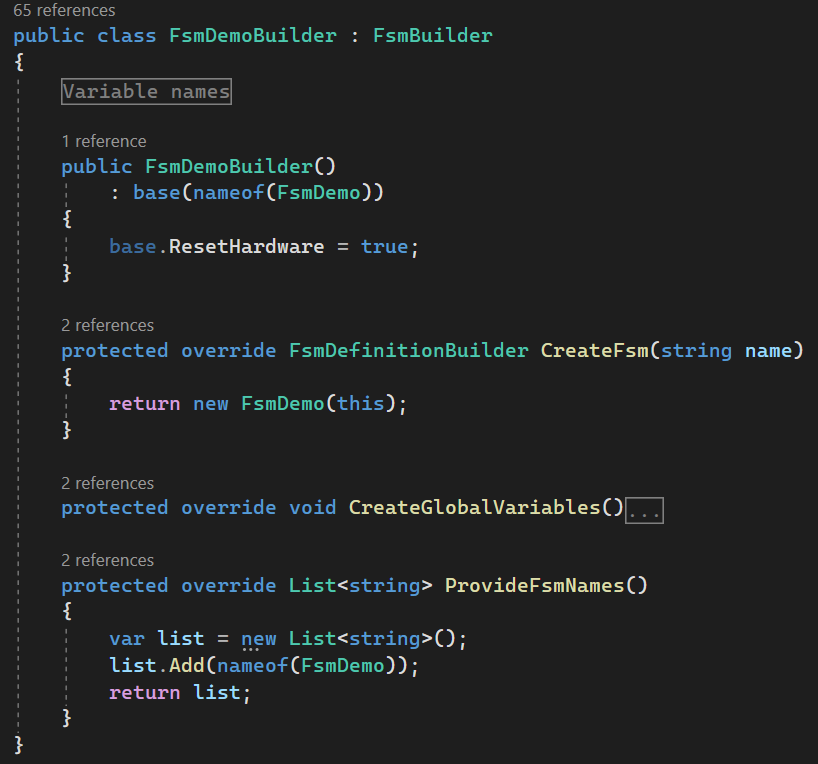
As shown to the right, The FsmBuilder is in turn inherited from a FsmDefinitionList, which is a collection of one or several independent state machine implementations.

The FsmDefinitionList also contains the variables in the global context (GlobalSignals).

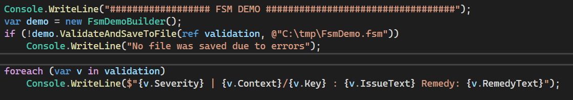
When the ValidateAndSaveToFile is called on the FsmBuilder to create a fsm-file, the FsmBuilder will first call CreateGlobalVariables, then ProvideFsmNames. Then, for each provided name, the FsmBuilder will call CreateFsm for each of them.

It is possible to have several state machines by returning more identifiers to the ProvideFsmNames (and of course their subsequent implementations when CreateFsm is called for each of the identifiers).

The CreateGlobalVariables method should create the hardware groups and the hardware signals towards the Accordion™ hardware. Here, it is also possible to add any other variable type that should be accessible from all state machines.

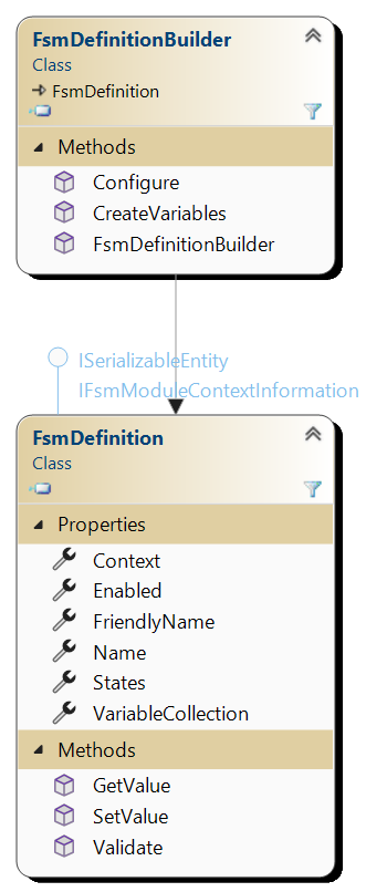
Next step is to provide the actual state machine implementation. As shown to the right, a FsmDefinitionBuilder inherits from the FsmDefinition class which provides the actual implementation of a state machine.

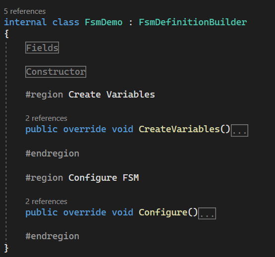
The constructor is called from the FsmBuilder (CreateFsm) and then CreateVariables and Configure methods are called sequentially for each defined FsmDefinition.

I

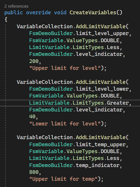
In CreateVariables, you should provide all the variables that this state machine needs.

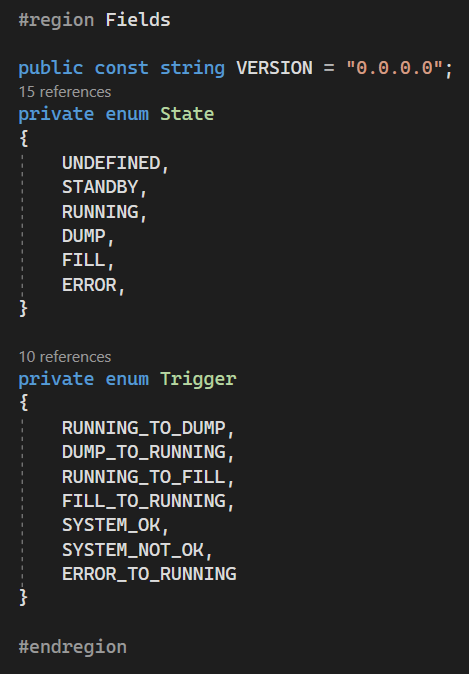
Now it is time to create all the states, actions and triggers. It is good practice to provide enums (or constant strings) for variable names, states and triggers. This reduces the chances for typos that will not be discovered until late in the development.

The provided names should be as descriptive as possible. The names you use will be visible in the state machine viewer as well as in the messages that streams from Accordion™ when running the state machine.

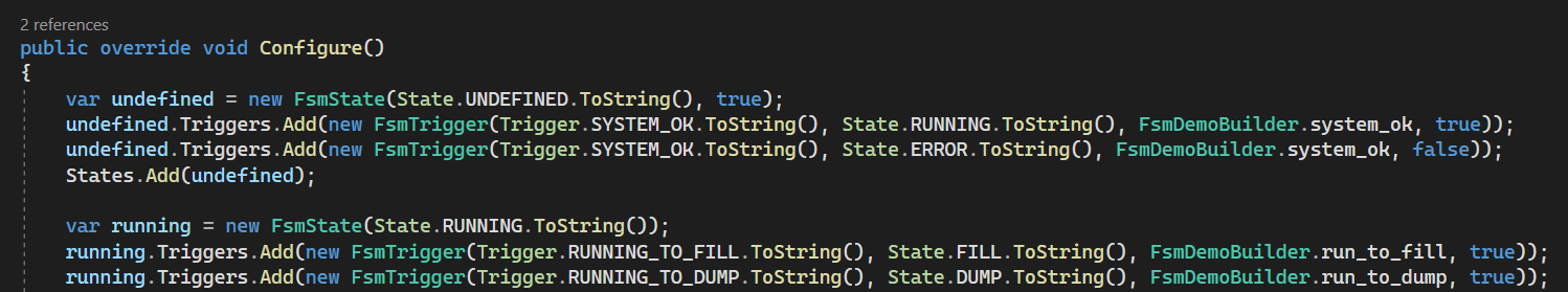
The Configure method should create all states, triggers and actions for the state machine.

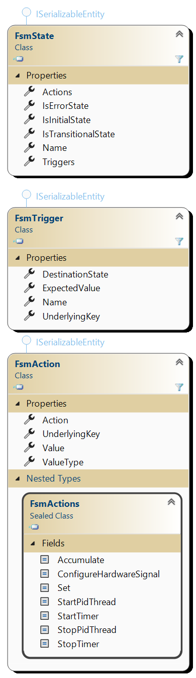
A FsmState is added to the States list. There’s no particular ordering required for the states.

A FsmState contains one or more FsmTriggers. At least one FsmTrigger is required, as otherwise the state would be a dead-end if it would enter such state.

A FsmTrigger defines a DestinationState. This name must match another FsmState in the same FsmDefinition. As the name implies, this is the state that should be transitioned to if the variable value of the UnderlyingKey is equal to the ExpectedValue.

A FsmState contains zero or more FsmActions. It is not necessary for a FsmState to contain actions, but a warning will be emitted as the state isn’t doing anything useful.

Every time the state machine transitions into a FsmState, all the defined FsmActions are performed.

A FsmAction defines an Action to be performed, which could be either of:

The UnderlyingKey contains the name of the variable to affect by this action and must be a variable name that exists either in the global context or the same context that the variable is created in.

Most Actions require a supplied Value (and a supplied ValueType). This is the value that will be assigned to the variable pointed out by the UnderlyingKey.

Implementation example

In this example, we want to build a pressure regulating machine that takes in temperature measurements and regulate the pressure based upon it. It is often useful to approach a state machine implementation in abstract terms as a state machine is really an abstraction of a machine.

On the physical hardware side we have two solenoid valves, one that increases the pressure in the system (fill valve) and one that decreases it (dump valve). We also have a temperature sensor that provides measurement data for the regulation. In addition we have a few safety features that needs to be considered, such as level- and temperature limits and an emergency stop button.

The simplest way to implement a process control is to just use a direct calculation:

if pressure > target => dump,

if pressure < target => fill

The problem with this implementation however is that it tends to oscillate between dumping and filling. Sometimes, it takes a while for a system to respond to changes (or even for the state machine to get the next measurement value that indicates the change it wanted).

In this case, we want to use a PID regulator where we can adjust the system response during validation without changing the logic.

So, our state machine should be continuously monitor all sensors and take action (dump, fill) if needed. We also want it to go to error if something bad happens.

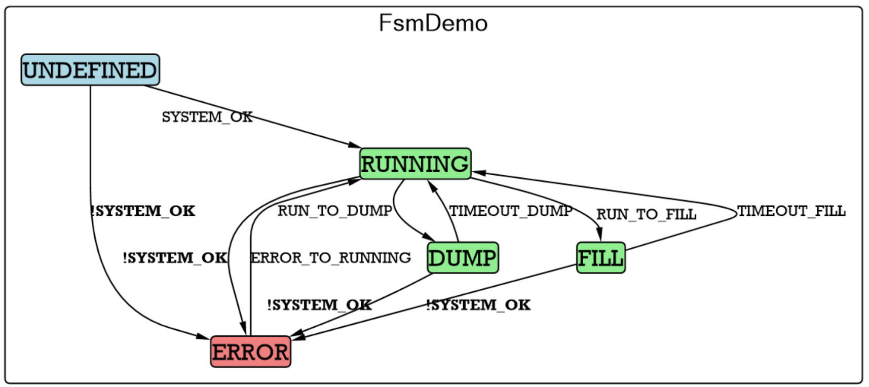
This state machine defines 5 states to complete the task:

• UNDEFINED: This is the initial state (where we start the whole operation). When the state machine loads, the variable SYSTEM_OK is evaluated. If it yields true, it will go to RUNNING, if it yields false, it will go to ERROR

• ERROR: All states have a transition into the ERROR state, each of them using a trigger SYSTEM_OK == false

• RUNNING: The stable state from which we either transition to DUMP or FILL depending on variables RUN_TO_DUMP and RUN_TO_FILL

• FILL/DUMP: Perform the fill/dump action and return to RUNNING when a timeout (TIMEOUT_FILL/TIMEOUT_DUMP) has elapsed.

Let’s first implement the states, triggers and actions for this abstract machine:

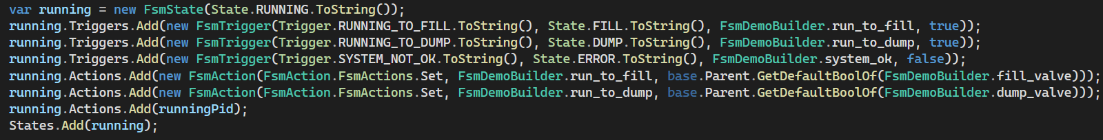
In the Configure() method:

Adding UNDEFINED state that triggers on SYSTEM_OK

Adding RUNNING state that either goes to FILL/DUMP if a variable is set or to ERROR if the SYSTEM_OK variable is false. It also turns off any fill/dump valves upon entry. The run_to_fill, run_to_dump variables should be regulated by a PID regulator, so we add a FsmPidAction here (runningPid) – more about this later.

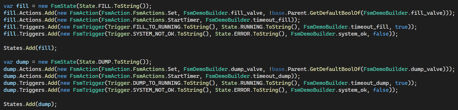
Adding FILL/DUMP states, which actuates the fill/dump valves respectively. It also starts a timer to transition back to the RUNNING state when elapsed. (The valves will be closed upon entering the RUNNING state).

Also these have an exit to ERROR if the SYSTEM_OK variable is false.

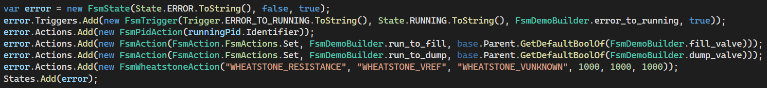
Lastly, adding the ERROR state

Now we have the states, the actions and the triggers in place, but nothing will really work yet. We now need to define the variables so the state machine knows how to evaluate things like SYSTEM_OK, or run_to_fill.

Let’s start with defining a variable for SYSTEM_OK:

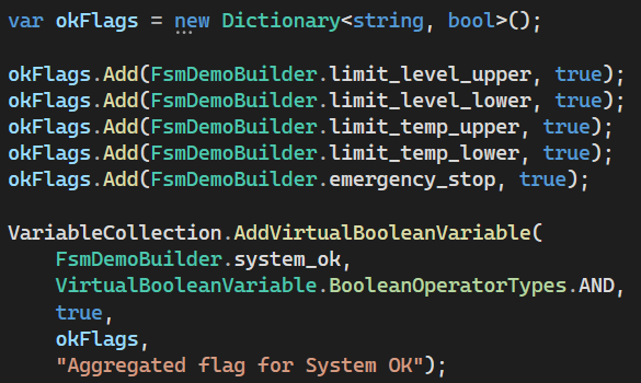
Here, we want to monitor both upper and lower limits of the fill level as well as the upper and lower limits of temperature. In addition, we want to monitor that the emergency stop hasn't been pressed. In the Dictionary, we add all these 5 variable names (we haven’t defined what they are yet) and create a VirtualBooleanVariable that should evaluate to true only if all of the variables are true (AND-condition).

Note the use of constant string fields here, to prevent misspelling.

Next step is to define the limits. Let’s take a look at the limit_level_upper as an example:

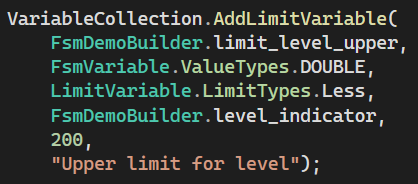
This adds a limit value with an underlying type of double that should be less than 200. It will evaluate this limit of 200 towards an underlying variable called level_indicator.

So, we need to add level_indicator to our variables collection:

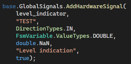
Our level_indicator is actually an analog pressure sensor that is connected to a MPIO signal on the Accordion™ hardware, which means there needs to be an entry in the alias translation file with this name:

For an analog signal, its gain and offset can be adjusted from the alias file. In this case, I have a ratiometric pressure sensor that converts 0-250 bar to 0.5-4.5V output voltage. To set the gain (Option 1), I have 250 bar range on a 4V signal => Gain=62.5 and a offset of 0.5V.

We also wanted a upper limit on the same level_indicator, which is added like this:

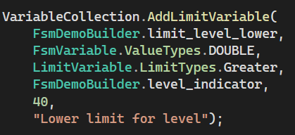
Each time the underlying variable (level_indicator) is updated, the limit variables will also update. If they change value, they will in turn update the dependent variable SYSTEM_OK.

The rest of the limits and sensor channels are added in the same fashion.

We now want to figure out a way to trigger a DUMP/FILL. We have defined run_to_fill and run_to_dump for this purpose; but what should control when these variables are set?

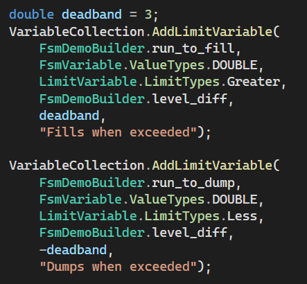
Here, the two variables are defined as LimitVariable’s, which will turn true if the underlying variable level_diff is either larger or less than the deadband. Within the deadband, both variables will be false.

Now, we also need a variable called level_diff. We want to calculate our desired pressure using a PID regulator. This desired pressure should be compared to our actual pressure and the difference between them is called level_diff.

As we want the difference between two values, we can use an OffsetVariable.

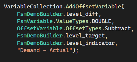
The level_diff will be equal to level_target – level_indicator. The variable level_target comes from our PID regulator, the level_indicator comes from a hardware signal that we added before.

Now, it is time to implement the creation of level_target. As this is the controller output of a PID regulator, let’s add it:

The prototype for a FsmPidAction is:

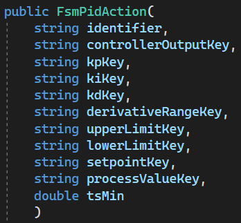
The identifier is an arbitrary name that identifies this PID regulator (you can define several), then we add the variable name level_target as the controller output as well as supplying all the other parameters a PID regulator needs.

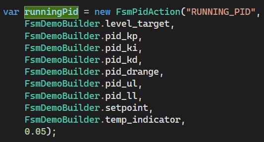
In principle, the PID regulator will monitor all the variables and will update the variable pointed out by the controllerOutputKey when the variable pointed out by processValueKey is updated. As our process value is the temp_indicator, a new level_target is calculated by the PID regulator each time temp_indicator is updated by the hardware.

Configuring and tuning a PID regulator (see Wikipedia) is a complex topic and not covered in this document, but a few tips and tricks are listed in the Frequently asked questions section.

State machine viewer

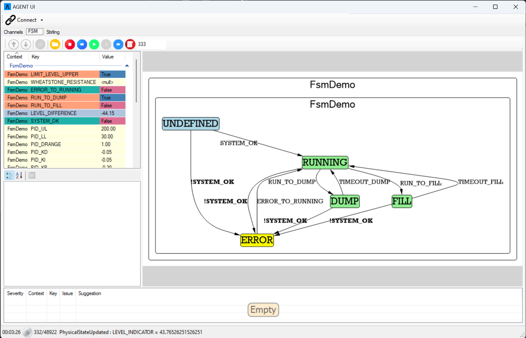
Once we have built a *.fsm file, it can be viewed in the built-in state machine viewer in AgentUI:

Start AgentUI, go to the “FSM” tab and press “Load File”:

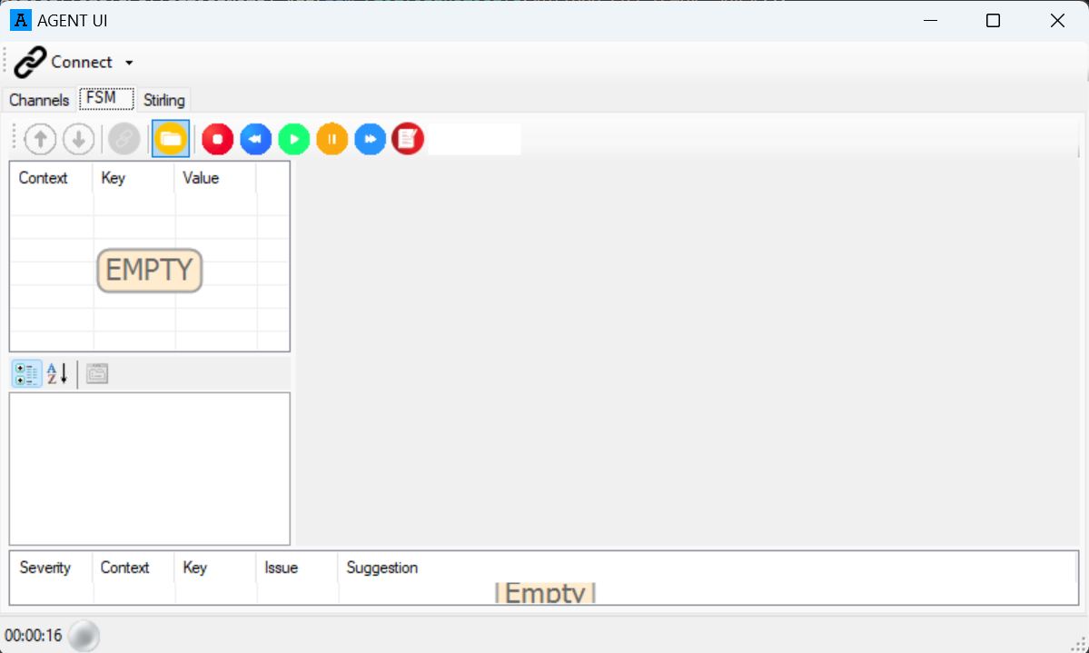
Once loaded, you will see the details of the state machine:

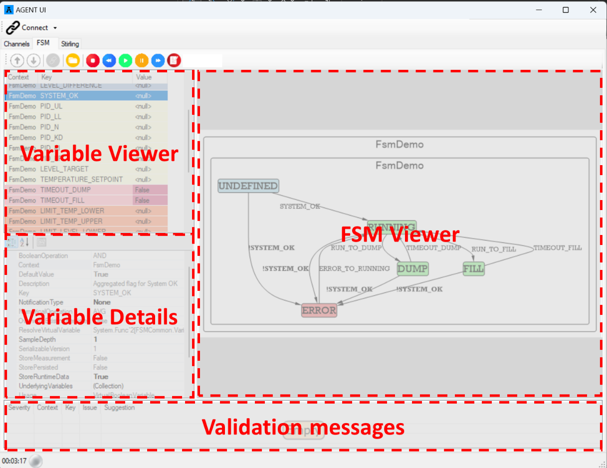
The variable viewer shows the list of all variables that you have defined. The variable type is distinguished by colors. Clicking a variable will bring up the variable details.

The FSM Viewer shows the states and transitions that are defined. Hovering over a state also reveals the actions associated with the state. Hovering over a transition reveals the transition settings.

In the bottom of the window, any validation messages from the Validation Engine is shown.

If the Accordion™ system is loaded with a state machine file, you could directly synchronize the view by pressing the button marked with an arrow.

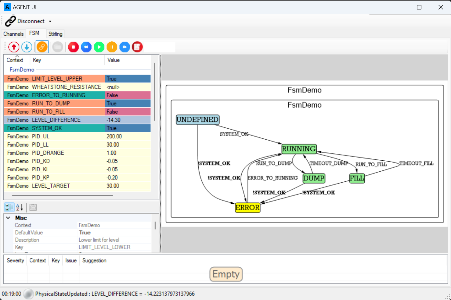
Once synchronized, all state transitions and variable values are automatically updated.

When AgentUI is running, all variables and states are recorded and stored at:

C:\Users\<user>\AppData\Local\AgentUI\AgentUI\<version>\<serial number>\<time-date>\

To view the recording, press the indicated button (Stop/Load) below and select the runtime session folder.

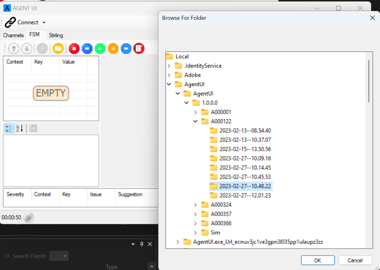
Once loaded, it shows the state machine definition and you can play/step/pause the recording.

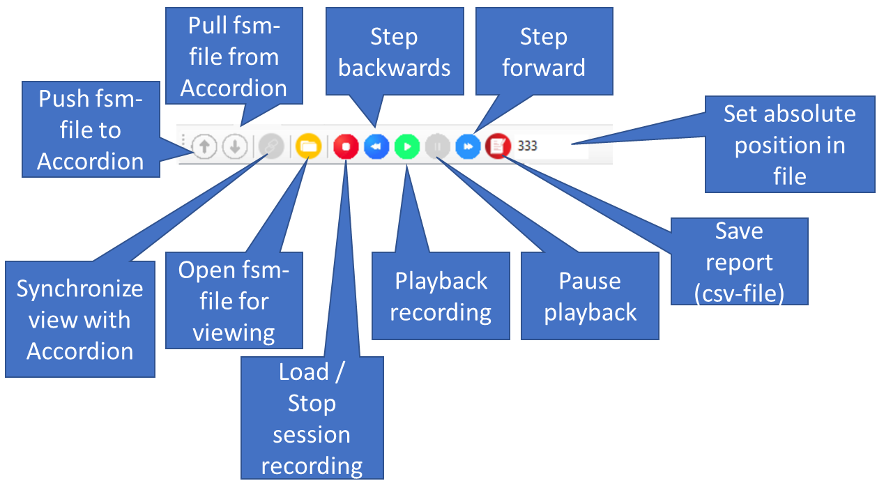
The “Save report” button will create a comma-separated file (.csv) in the same directory as the ‘states.step’ file is located. All variables defined in the FSM will be representedas 2-dimensional data that can be post-processed in Excel.

Validation Engine

The validation engine provides extensive validation of the created state machine. It will either emit a recommendation, warning, or error in case it encounters a questionable statement or item. The validation is shown both during creation, but also if you load the file in AgentUI. Note that if errors are encountered, no file will be created unless the flag saveDespiteErrors is set.

An Error is defined as something that is guaranteed to not work when running. It could for example be dead states (states that doesn’t have a transition into it), states that are a dead-end (state lacking a transition out from it), defined triggers that references variables that don’t exist or recursive variables that will cause stack overflow.

A Warning is defined as something that is probably wrong, but if you know what you are doing, you can disregard them. Warnings are typically emitted if you define states that doesn’t do anything (zero actions) or if you duplicate actions or triggers.

A Recommendation is defined as something you might want to reconsider in your design. For example defining variables that are unused.

Frequently asked questions

How do I configure hardware signals?

Please consult the Agent manual.

How do I make a composite boolean expression, such as [(a & !b) || (!a & c)]?

Create three VirtualBooleanVariable’s:

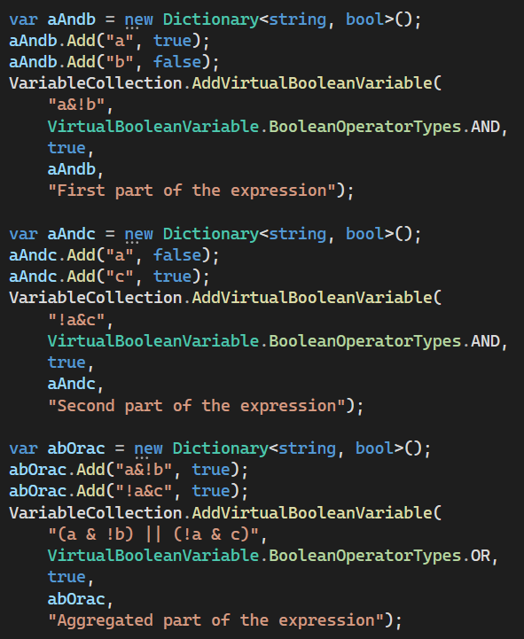
How do I tune PID parameters?

Configuring an tuning a PID regulator (see Wikipedia) is a complex topic, but there are a few approaches listed on the Wikipedia page. But one can get decent start values by thinking about the representation of the process value and the controller output. Also the sampling time is critical in finding the correct tuning values.

Let’s say the process value is a temperature that you want to keep as close as 700°C as you can (setpoint). The controller output is a pressure, which is somewhere between 32-200 bar. You measure the temperature with a frequency of 1Hz (interval=1000).

First, you assign the upper- and lower limits to 32/200 and the setpoint to 700.

Considering KP:

Think about what you want to happen with the pressure if the temperature is, say, +10% above the setpoint: Perhaps you then want the pressure to rise with about 1%. That means that for a process value difference of 700-770=-70°C, you want to accumulate 1% of the controller output which spans from 32-200. The range is then 200-32=>168 bar and 1% of that is 1.68 bar. KP should then be fulfilling the equation:

1.68 = KP * -70 => -0.024 (KP)

Note the sign here, an error of -70 should be giving a higher pressure, hence the KP term must be negative.

Considering KI:

Sometimes proportional gain KP isn’t enough to push the machine to the desired value. The effect of KP will approach zero when the error approaches zero. If this is the case, you can consider adding integral gain. As the name suggests, it integrates the error and after a while the error signal will be sufficiently high to cause a change in pressure. Note that integrating the error when the process value stays far away from the setpoint during a long time can cause this integration to be very high (integral wind-up). The PID implementation in SME prevents this by zeroing the integral error when the output clamps to either limit.

Typically, you want KP to do the heavy lifting when far away from the setpoint and let the KI play a role when the error is close to zero. This implies that the KI term should be much smaller than the KP term (in our example -0.024). Here, sample time plays a big role, and we had set the sampling time of the temperature to 1Hz (once per second).

The PID regulator uses the following equation:

IntegralTerm += (Ki * Error * Ts) (where Ts is the time in seconds)

So for an error of -70°C and Ts=1, the integral term would wind up and clamp very fast unless the Ki parameter is very small.

Let’s say that it is reasonable that for a error of 0.1% (-7°C in our example), we want to slowly increase the error signal by 0.005% (8.4mbar per second)

0.0084 = KI * -7 => -0.0012 (KI)

Considering KD:

You can use the derivative term if you want to limit the rate of change of the data, regardless of the setpoint. This gives the controller “predictive” capabilities, meaning that it can limit the rate when the process value approaches the setpoint. However, using a derivative term could easily push the controller to be unstable and in many applications you will probably give up and set the KD = 0 to achieve a stable behavior.

To make the KD term slightly more usable, the implementation in SME uses a setting DerivativeRange, which sets the maximum contribution that the derivative term can apply.

Looking at a PID regulator response can aid in understanding how to adjust parameters to get the behavior you want. In this case, we are aiming for 650°C (process value) by adjusting the pressure (controller output).

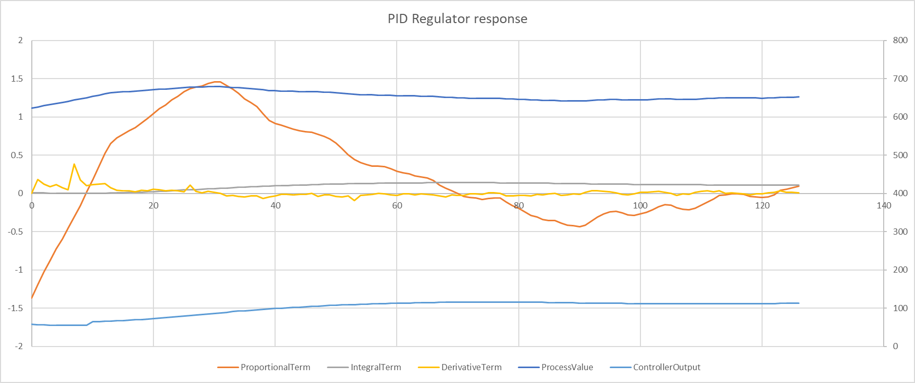
To the left, the temperature is lower than the setpoint, and the proportional term has a relatively high negative contribution. At the same time, the temperature is approaching the setpoint fast and the proportional term is somewhat negated by the positive value from the derivative term. Essentially, the derivative term tries to “brake” the fast response that the proportional term otherwise would yield. After this initial contribution, the derivative term is negligible as the rate of change is so low.

Once the error is pulled to a low value, the integral term slowly pushes up the value to reach the optimum temperature. Here, the proportional term is so small, so it doesn’t really affect the controller output that much.

My analog signal is noisy, how do I filter it?

Use the numerical operation Average and set the sample depth to an appropriate value.

(The numerical operation is Average by default)

I want to count the number of times a state is visited, how do I do that?

Create a VirtualVariable and let the action FsmAccumulationAction do the work.

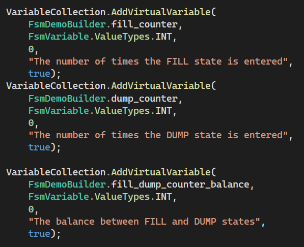
Example, we want to count the number of times the states DUMP and FILL is entered. We also want to know the balance of the calls such that if FILL and DUMP is called an equal amount of times, the balance is zero.

First add VirtualVariable’s that will hold the values:

Then, in the state actions, add appropriate FsmAccumulationAction’s:

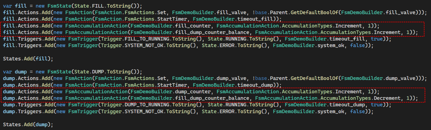
Each time the FILL state is entered, the fill_counter is incremented by one and the fill_dump_counter_balance is incremented by one.

Each time the DUMP state is entered, the dump_counter is incremented by one and the fill_dump_counter_balance is decremented by one.